Directory UMM :Data Elmu:jurnal:I:International Review of Economics And Finance:Vol8.Issue4.Nov1999:

(1)

International Review of Economics and Finance 8 (1999) 375–397

The intraday relation between return volatility,

transactions, and volume

✩

Xiaoqing Eleanor Xu

a

_{, Chunchi Wu}

b,

_*

a_{School of Business and Administration, St. Louis University, 3674 Lindell Blvd., St. Louis, MO 63108, USA}

b_{School of Management, Syracuse University, Syracuse, NY 13244-2130, USA}

Received 5 February 1998; accepted 16 July 1998

Abstract

In this article, we examine the relation between return volatility, average trade size, and the frequency of transactions using transaction data. Consistent with Jones, Kaul, and Lipson (1994.Review of Financial Studies, 7, 631–651), our results show that the frequency of trades has a high explanatory power for return volatility. However, contrary to their finding, we find that average trade size contains nontrivial information for return volatility. The positive relation between return volatility and average trade size is more significant for actively traded stocks. Furthermore, return volatility exhibits significant intraday variations. It is found that the effect of trade frequency on return volatility is much stronger in the opening trading period. 1999 Elsevier Science Inc. All rights reserved.

JEL classification:G10; D82

Keywords:Information asymmetry; Trade size; Frequency

1. Introduction

Financial researchers have paid a great deal of attention to the relation between trading volume and stock return volatility. Empirical studies have generally found a positive relation between return volatility and transaction volume.1 _{Karpoff (1987)} conducted a comprehensive survey on the relation between price changes and trading volume. Schwert (1989), Gallant et al. (1992), and Foster and Viswanathan (1993) found a positive correlation between stock return volatility and trading volume.

The positive correlation between volatility and volume supports the Mixture of

✩_{An earlier version of this paper was presented at the 1997 Eastern Finance Association Meetings.}

* Corresponding author. Tel.: 315-443-3549; fax: 315-443-5389.

E-mail address: cwu@syr.edu (C. Wu)

(2)

← →

376 X.E. Xu, C. Wu / International Review of Economics and Finance 8 (1999) 375–397

Distribution Hypothesis (MDH). Originally developed by Clark (1973) and subse-quently extended by Tauchen and Pitts (1983), Lamoureux and Lastrapes (1990), and Anderson (1996), the MDH postulates that return volatility and volume are positively correlated because both are related to the underlying information flow. The strong contemporaneous correlation between trading volume and return volatility docu-mented by previous studies may well reflect their joint dependence on the underlying latent events.

Recently, Jones, Kaul, and Lipson (1994; hereafter JKL) documented striking evi-dence for the role of the frequency of trades in determining the volatility of returns. They found that the positive relation between volatility and volume actually reflects the positive relation between volatility and the frequency of transactions.2 _{On the} other hand, the size of trades has virtually no information beyond that contained in the frequency of transactions. Based on this finding, they concluded that the number of transactions contains all the pertinent information to the pricing of securities.

The finding that the size of trades contains no information is puzzling. Financial theories, represented by both the competitive and strategic models, have predicted a positive correlation between the size of trades and volatility. In competitive models (Pfleiderer, 1984; Grundy & McNichols, 1989; Holthausen & Verrecchia, 1990; Kim & Verrecchia, 1991), the trade size is shown to be positively related to the quality of information, and insiders prefer to trade a large size at any given price. In strategic models with a monopoly informed trader (Kyle, 1985; Admati & Pfleiderer, 1988; Foster & Viswanathan, 1990), a camouflage of one large trade into several small-sized trades tends to obscure the relation between volatility and trading size. However, in a more realistic setting with multiple informed traders, Holden and Subrahmanyam (1992) showed a similar positive relation between trading size and the quality of information possessed by informed traders. Thus, both competitive and strategic mod-els predict a positive relation between the size of trades of informed traders and the quality of their information and hence a positive relation between average trade size and price changes. The predictions of these theoretical models are apparently at odds with JKL’s finding.

Furthermore, it has often been argued that it takes volume to move prices. Technical securities analysts use volume data extensively to predict future price movements. Grundy and McNichols (1989) demonstrated the informational role of volume and its applicability for technical analysis. Blume et al. (1994) showed how trading volume, information precision, and price fluctuations are related. They found that traders who use the information contained in volume obtain higher-quality private signals than traders who do not. The finding that average trade size contains no information would seem to be inconsistent with the volume-based technical trading activities observed in security markets.

(3)

X.E. Xu, C. Wu / International Review of Economics and Finance 8 (1999) 375–397 377

theory. A main objective of our study is to see if JKL’s results hold at the intraday interval. Also, it will be interesting to see whether the volatility–transaction relation varies over intraday periods.

Second, we use the generalized method of moments (GMM) in empirical estimation. The GMM model invokes much weaker distributional assumptions on stock returns. Within the GMM framework, the disturbance terms of the volatility regressions can be both serially correlated and conditionally heteroskedastic. The GMM thus provides more robust tests than least squares regressions that rely heavily on the assumption of serial independence and homoskedasticity. Because returns and volatility are poten-tially correlated across firms, we jointly estimate the parameters of the volatility model for the system of equations involving all firms in the sample. By taking into account cross-sectional correlation between individual firms, we obtain an efficient estimate of the regression parameter.

Third, in empirical estimation we introduce an ad hoc adjustment for camouflaged trades, where one transaction may be strategically split into several trades to minimize their impact on market price. Order splitting tends to attenuate the relation between return volatility and average trade size while boosting the effect of trade frequency. To mitigate this effect, we adjust the frequency and size of trades reported in the raw data to account for the effect of camouflaged trades.

Our result shows that the frequency of transaction significantly affects intraday return volatility. This result is consistent with JKL’s finding based on the interday data. In addition, our study documents several interesting findings. First, we found that the size of trade is significantly related to return volatility, particularly for more frequently traded stocks. Because trade frequency is positively correlated with firm size, the size of trade is also positively related with return volatility of large firms. This result contrasts JKL’s interday finding that there is virtually no positive relation between average trade size and return volatility for large firms. Second, we found significant variations in the transaction–volatility relation over the intraday periods. Consistent with Wood et al. (1985), Jain and Joh (1988), and Stoll and Whaley (1990), we found that stock return volatility varies over intraday intervals, with the highest volatility occurring at the opening of the market. Moreover, we found that the effect of the frequency of trades on return volatility is much stronger in the market opening period. Finally, we provide some evidence that order splitting tends to attenuate the empirical relation between average trade size and return volatility, while boosting the effect of trading frequency on return volatility.

The remainder of this article is organized as follows. In section 2, we describe the model and estimation problems. We discuss the time pattern of return volatility and possible variations in the volatility–volume relation over the intraday periods. In section 3, we describe the empirical methodology and estimation procedures. We then discuss our data and present our results in section 4. Finally, we summarize our findings in section 5.

2. The model

(4)

← →

volatility as the absolute percentage price change conditional on past returns and day-of-the-week effects. Specifically, we first estimate the residual of the following return model:

where Rit is the return of security i over a half-hour interval t; Wkt’s are weekday

indicator variables;Rit2nis the return of securityiat time t2n; andeitis the residual

of securityi.4_{Similar to JKL (1994), lagged (14) half-hourly returns are used to capture} the short-term movements in conditional expected returns. We then multiply the absolute residual from the above model, |eit|, by 1,000 and use it as a measure of

return volatility (VOLit) of securityiin period t.

Return volatility for each stock is then regressed against its frequency of transactions (NT), average trade size (ATS), the dummy variables for the first half hour (OPEN) and the closing half hour (CLOSE), Monday dummy (MONDAY), and 14 lagged volatility terms. Specifically, we estimate the following volatility regression:

VOLit5 ai1 giATSit 1 biNTit 1 hiOPENt1 viCLOSEt1 piMONDAYt

1

_o

14

n51

linVOLit2n 1 mit (2)

wheremit is the disturbance term.

Wood et al. (1985) and Jain and Joh (1988) documented that NYSE trading volume follows a U-shaped intraday pattern. In addition, Stoll and Whaley (1990) and Foster and Viswanathan (1993) show that the volatility at market opening is much higher because of asymmetry information effects arising from non-trading overnight. The half-hourly dummy variables OPEN and CLOSE in the above regression model are used to detect any differences in intraday return volatility in the opening and closing intervals after accounting for the information content in volume. The Monday dummy variable is introduced to reflect the trading-gap effect at the beginning of the week. This dummy variable equals 1 for Mondays and 0 otherwise. Thelcoefficients reflect the persistence in the volatility of securityi.The lagged VOL terms for each security are included to correct for heteroskedasticity in return volatility.

As the pattern of intraday return volatility varies over time, the volatility–volume relation may differ across intraday trading periods. To examine whether the relation of return volatility with the frequency of transactions and average trade size changes over intraday periods, we also estimate the following regression:

VOLit5 ai1 giATSit 1 biNTit 1 hiOPENt3ATSit 1 viOPENt3NTit

1 piMONDAYt 1

o

14

n51

linVOLit2n 1 mit (2a)

(5)

Another issue is related to the specification in the volatility regression. In JKL’s study, they separated volume into the components of average trade size and the number of transactions. The average trade size is defined as the total number of shares traded in a period (day) divided by the number of transactions. By definition, total trading volume is simply the product of average trade size and the number of transac-tions. Thus, one cannot linearly separate total trading volume into these two compo-nents. One possible consequence is that the total effect of trading volume may not be completely captured by the sum of the effects of the size and frequency of trades. An alternative specification is to take a log transformation of each transaction variable so that the log total volume is exactly equal to the sum of the log values of average trade size and the number of transactions. In principle, this log transformation may provide a better decomposition of the total volume effect. In our empirical investiga-tion, we use the variables of size and frequency of trades with and without the log transformation and examine the sensitivity of estimation results to these variable specifications.

3. Empirical methodology

We use the GMM method for empirical estimation (Hansen, 1982). The GMM requires much weaker distributional assumptions than other estimation methods. It is therefore especially suitable for estimating a model that may not satisfy some regularity conditions of least squares. It is well known that heteroskedasticity of return volatility is a pervasive phenomenon both at the individual security and portfolio levels.6_{Also, in the present case, the volatility measure is essentially the conditional} absolute returns, which may be subject to serial correlation.7_{The GMM provides a} more robust framework for parameter estimation and hypothesis tests in the presence of both statistical problems.

The GMM estimation involves specifying a set of moment conditions. For example, for each individual regression specified in Eq. (2), the following orthogonal conditions must be satisfied:

E(mt) 50

E(mtATSt) 50

E(mtNTt) 50

E(mtOPENt)5 0

E(mtCLOSEt) 50

E(mtMONDAYt) 50

E(mtVOLt2j) 5 0,j5 1, 2, . . . , 14. (3)

These conditions state that the expected cross products of unobservable distur-bances, mt, and the explanatory variables are equal to 0. The first moment of the

cross-products is:

mN (u) 5

1 N

o

N

t51

(6)

← →

where Zt is a vector of variables included in the regression model, u is a vector of

parameters to be estimated,Nis the number of observations, and the disturbancemt

is stationary. For each regression, there are 20 orthogonal conditions and 20 parameters to be estimated.8_{For example, for 141 cross-sectional units, there are a total of 141}₃ 2052,820 parameters to be estimated. Since the number of parameters to be estimated equals the number of orthogonal conditions, the model is just identified.

We estimate the true parameter vector u0 by the value of uˆ that minimizes the following quadratic function:

S(u,V) 5[NmN(u)]9V21[NmN(u)]9 (5)

where

V5Cov([NmN(u0)],[NmN(u0)]9).

We impose the moment condition [Eq. (3)] in estimating the volatility regressions of individual securities. The procedure of the GMM estimation involves selecting an estimator to set the linear combination of the moment conditions to 0 while minimizing [Eq. (5)]. We apply the GMM to the system of equations involving all securities in the sample. More specifically, we estimate Eqs. (2) or (2a) simultaneously for all securities to provide efficient estimates of parameters by accounting for cross-correla-tion in error terms.

4. Data and empirical results

Data for price, size, time, and date for each stock transaction were obtained from the Trades and Quotes (TAQ) database of the New York Stock Exchange (NYSE) over the period from April to June 1995. Over this period, the NYSE was open from 9:30 a.m. to 4:00 p.m. Eastern Time. Transaction data in each day are divided evenly into 13 half-hour intervals for 63 trading days. This results in 819 time series units (observations) for each stock. We use the midquotes at the beginning and the end of each 30-minute interval to compute the returns for each stock for that interval. Using midquotes avoids measurement errors caused by bid-ask bounce, which induce spuri-ous volatility in stock returns. For each half-hour interval, we count the number of transactions and calculate the average trade size for each stock. Average trade size and the number of trades are all assumed to be 0 for no-trade intervals.

The sample includes 141 randomly selected stocks from the TAQ database.9 _We

(7)

4.1. Empirical evidence

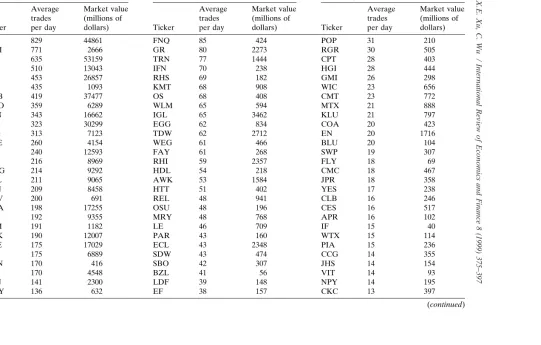
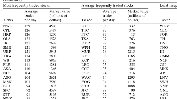
Table 1 lists the firms (ticks) included in the sample by the order of average daily trading frequency, and summarizes the characteristics of stocks included in the sample. As shown in Table 1, there is a sharp difference in the average frequency of trades between the three groups of stocks. The average daily number of transactions is 229 for the most frequently traded stocks, whereas it averages only 16 transactions per day for the least traded stocks. The average market values of the firms at the end of the second quarter of 1995 are reported in the last column. As expected, the trade frequency is positively correlated with firm size.

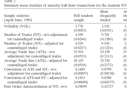
The cross-sectional average and standard error of firm-specific intraday trade statis-tics at 30-minute intervals (i.e., volatility [VOL], the number of trades [NT], average trade size [ATS], correlation between ATS and NT, and the first-order autocorrelation of NT and ATS) are provided in Table 2. The volatility, average trade size, and the number of trades are all higher for more frequently traded stocks. Not surprisingly, the number of trades is lower, while the average trade size is higher after the adjustment for camouflaged trades. The low correlation between NT and ATS ensures that there is no serious multicollinearity between NT and ATS in the regression. The first-order autocorrelation of ATS is about 0.06, while that of NT is 0.29.

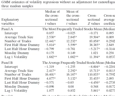
For brevity, we only report the results of estimation for the volatility–volume regressions.10 _{Table 3 summarizes the results of volatility regressions for the entire} sample without an adjustment for camouflaged trades. Columns 2–4 include the cross-sectional median, mean of thetstatistics of parameter estimates, and theirZstatistics.11 Columns 5 and 6 show the average coefficient estimates and their test statistics (T), which measure the significance of the respective aggregate estimates.12 _{The pattern} for the coefficient estimates of the number (frequency) of transactions is quite similar

to those obtained by JKL. The average t value for the number of transactions is

relatively large (15.210) and significant at the 1% level. However, contrary to JKL’s finding, the averagetvalue for average trade size is 2.018, which is significant at the 5% level. The Z statistic for the average trade size is 23.962, which shows an even stronger result for the importance of average trade size in explaining the return volatility at intraday hour–hour intervals. The aggregateTstatistics exhibit a similar pattern with the coefficients of both the size and frequency of trades being significant at the 1% level.

Empirical results from the full sample indicate that the number of trades and average trade size both have significant relationships with the return volatility. However, the impact of changes in the number of trades on return volatility is still stronger than that on average trade size. The average coefficient for NT is 0.761, which indicates that one standard deviation increase in NT (i.e., 3.407 trades) would result in a 2.593 unit increase in return volatility. On the other hand, the average coefficient for ATS is 0.0076, indicating a 0.240 unit increase in return volatility for each standard deviation increase in ATS (i.e., 31.544 hundred shares).

(8)

←

The TAQ random NYSE sample: 141 stocks

Most frequently traded stocks Average frequently traded stocks Least frequently traded stocks

Average Market value Average Market value Average Market value

trades (millions of trades (millions of trades (millions of

Ticker per day dollars) Ticker per day dollars) Ticker per day dollars)

DIS 829 44861 FNQ 85 424 POP 31 210

NSM 771 2666 GR 80 2273 RGR 30 505

PFE 635 53159 TRN 77 1444 CPT 28 403

ATI 510 13043 IFN 70 238 HGI 28 444

TX 453 26857 RHS 69 182 GMI 26 298

UIS 435 1093 KMT 68 908 WIC 23 656

CMB 419 37477 OS 68 408 CMT 23 772

MRO 359 6289 WLM 65 594 MTX 21 888

FON 343 16662 IGL 65 3462 KLU 21 797

AIT 323 30299 EGG 62 834 COA 20 423

SEG 313 7123 TDW 62 2712 EN 20 1716

NUE 260 4154 WEG 61 466 BLU 20 104

BK 240 12593 FAY 61 268 SWP 19 307

GIS 216 8969 RHI 59 2357 FLY 18 69

WAG 214 9292 HDL 54 218 CMC 18 467

UCL 211 9065 AWK 53 1584 JPR 18 358

TEN 209 8458 HTT 51 402 YES 17 238

NAV 200 691 REL 48 941 CLB 16 246

WLA 198 17255 OSU 48 196 CES 16 517

CSX 192 9355 MRY 48 768 APR 16 102

SRM 191 1182 LE 46 709 IF 15 40

ROK 190 12007 PAR 43 160 WTX 15 114

NKE 175 17029 ECL 43 2348 PIA 15 236

(9)

→

Most frequently traded stocks Average frequently traded stocks Least frequently traded stocks

Average Market value Average Market value Average Market value

trades (millions of trades (millions of trades (millions of

Ticker per day dollars) Ticker per day dollars) Ticker per day dollars)

NWL 129 4506 DUC 38 332 WDV 13 88

Sample No. of stocks number of trades (millions of dollars)

Most frequently traded stocks 47 229 9191.28

Average frequently traded stocks 47 48 910.42

Least frequently traded stocks 47 16 311.55

(10)

← →

Table 2

Summary mean statistics of intraday half-hour transactions for the random NYSE sample

Most Average Least

Sample statistics Full random frequently frequently frequently

(April-June, 1995) sample traded traded traded

Volatility (VOL) 1.770 2.552 1.993 0.825

(0.0052) (0.0191) (0.0179) (0.0072)

Number of Trades (NT)—w/o adjustment 4.399 9.701 2.585 0.910

for camouflaged trades (0.0244) (0.1260) (0.0202) (0.0078)

Number of Trades (NT)—adjusted for 4.339 9.543 2.566 0.908

camouflaged trades (0.0237) (0.1224) (0.0199) (0.0078)

Average Trade Size (ATS)—w/o 15.934 25.359 15.425 7.017

adjustment for camouflaged trades (0.0553) (0.2113) (0.1705) (0.1009) Average Trade Size (ATS)—adjusted for 16.129 25.783 15.557 7.047

Correlation of ATS and NT—w/o 0.1849 0.0799 0.1556 0.3154

adjustment for camouflaged trades (0.00097) (0.00156) (0.00167) (0.00272) Correlation of ATS and NT—adjusted for 0.1833 0.0786 0.1553 0.3159

First Order Autocorrelation of NT—w/o 0.29099 0.41727 0.30581 0.15537 adjustment for camouflaged trades (0.00126) (0.00304) (0.00356) (0.00249) First Order Autocorrelation of NT— 0.29177 0.41640 0.30453 0.15438

adjusted for camouflaged trades (0.00127) (0.00304) (0.00355) (0.00248) First Order Autocorrelation of ATS— 0.05703 0.07338 0.05049 0.04629

w/o adjustment for camouflaged trades (0.00041) (0.00142) (0.00121) (0.00101) First Order Autocorrelation of ATS— 0.05626 0.07070 0.05162 0.04645

adjusted for camouflaged trades (0.00040) (0.00133) (0.00120) (0.04717) This table reports the cross-sectional average of firm-specific intraday 30-minute interval trade statistics (with the standard error of the cross-sectional average in parentheses). VOL (stock return volatility measure) is the absolute value of the return conditional on its 14 lags and weekday dummies; NT (Number of Trades) is the number of NYSE transactions for each 30-minute trading period; and ATS (Average Trade Size) is the mean number of shares (in hundreds) traded per transaction for each 30-minute interval.

half hour is not significant. We also checked the volatility pattern for other intraday trading periods. None of the remaining trading intervals has a significant dummy coefficient. Thus, after considering the volume effects, it appears that only the opening half hour exhibits a unique pattern of volatility.

(11)

X.E. Xu, C. Wu / International Review of Economics and Finance 8 (1999) 375–397 385 Table 3

GMM estimates of volatility regressions without an adjustment for camouflaged trades: The full sample Median of Mean of

the cross- the cross- Cross- Cross-sectional Tvalues of

Explanatory sectional sectional sectional average the average

variables tvalues tvalues Zvalues coefficients coefficients

Intercept 21.337 21.281 215.211* 20.1432 23.3072*

Average Trade Size 1.942** 2.018* 23.962* 0.0076 6.2975*

Number of Trades 14.900* 15.210* 180.609* 0.761 14.4677*

First Half Hour Dummy 4.144* 4.306* 51.131* 1.786 10.5059*

Last Half Hour Dummy 20.653 20.664 27.885* 20.2579 27.2648*

Monday Dummy 20.074 0.02 0.237 0.0839 0.9051

Lag 1 Volatility 0.891 1.009 11.981* 0.0324 6.3720*

Lag 2 Volatility 20.075 0.056 0.665 0.0016 0.5842

Lag 3 Volatility 20.002 0.108 1.282 0.0029 0.9832

Lag 4 Volatility 20.064 0.089 1.057 0.0032 1.0557

Lag 5 Volatility 0.11 0.301 3.574* 0.0091 2.4543*

Lag 6 Volatility 0.087 0.102 1.211 0.0032 1.2299

Lag 7 Volatility 0.251 0.246 2.921* 0.008 2.2914*

Lag 8 Volatility 20.054 0.073 0.867 0.0024 0.6847

Lag 9 Volatility 20.327 20.087 21.033 20.0027 20.9331

Lag 10 Volatility 20.097 20.032 20.380 20.0006 20.1778

Lag 11 Volatility 0.222 0.26 3.087* 0.0074 2.5188*

Lag 12 Volatility 0.276 0.294 3.491* 0.0088 3.5749*

Lag 13 Volatility 20.171 0.042 0.499 0.0013 0.4693

Lag 14 Volatility 20.205 20.055 20.653 20.0016 20.5688

Estimates of the following regression for the full random sample (141 stocks): VOLit5 ai1 giAVit1 biNTit1 hiOPENt1 viCLOSEt1 piMONDAYt1

o

14

n51

linVOLit2n1 mit

where VOLit(stock return volatility measure) is the absolute value of the return on securityiat timet

conditional on its 14 lags and weekday dummies, NTitis the number of transactions for securityiat time

t, ATSitis the average trade size (total share volume divided by the number of transactions) for security

iat timet, OPENtis a dummy variable that is equal to 1 for the open half hour and 0 otherwise, CLOSEt is a dummy variable that is equal to 1 for the close half hour and 0 otherwise, MONDAYtis a dummy variable that is equal to 1 for Mondays and 0 otherwise, and the coefficientslinmeasure the persistence in volatility of securityi. The sample period is from April 1995 to June 1995. Each regression has 819 time series observations. * indicates a significance level of 5% or better for two-tailed test whereas ** indicates a significance level of 5% for one-tailed test. The cross-sectionalZvalue in the column 4 is calculated as the meantvalue multiplied by√141. The Tvalue in the last column is calculated as the cross-sectional average coefficient in column 5 divided by the standard error of the cross-sectional coefficient. Mean (Median)R2₅_{32.77% (32.61%).}

(12)

← →

at the 5% level. Again, contrary to JKL’s finding, average trade size appears to contain a significant amount of information. TheZandTvalues further support this hypothesis. Table 4 (panel C) reports the results for the stocks with the lowest frequency of trades. Interestingly, the results for this group are much closer to the finding of JKL’s study. The coefficient of the number (frequency) of transactions is highly significant, whereas the coefficient of average trade size is not significant. However, the mean coefficient of average trade size is still positive, and thetstatistics are significant for a little more than 25% of the stocks in this group. The Zstatistics and aggregate T statistics show a similar pattern of statistical significance for both average trade size and frequency.

It is worth noting that the average daily number of transactions is quite small for the least traded group, as shown in Table 1. Although the asymmetric information effect at transaction level might be stronger for infrequently traded stocks (see Easley et al., 1996), the contemporaneoushalf-hour return volatility–size effect is shown to be weaker than that of more frequently traded stocks. One possible reason behind this perplexing result is that infrequently traded stocks typically have a slower price discovery process. Also, from the empirical standpoint, infrequent trading produces a data discreteness problem in the estimation. This problem could cause the estimates of the average trade size coefficient to be biased toward 0 for the infrequently traded stocks. This statistical problem associated with infrequent trading is well documented in the finance literature (e.g., Campbell et al., 1997). The problem of infrequent trading or non-trading tends to obscure the empirical relation between volatility and average trade size.

The average coefficients differ significantly across the three sub-samples. For in-stance, one standard deviation change in average trade size would result in a 0.330 unit change in volatility for the most frequently traded stocks, 0.417 for the average frequently traded stocks, and 0.052 for the least frequently traded stocks. On the other hand, one standard deviation change in the number of trades would result in a 1.599 unit change in volatility for the most frequently traded stocks, 1.992 for the average frequently traded stocks, and 1.537 for the least frequently traded stocks. The impact of changes in the number of trades on volatility is generally stronger than the impact of changes in average trade size. Also, the impact of average trade size on volatility appears to be much weaker for least frequently traded stocks.

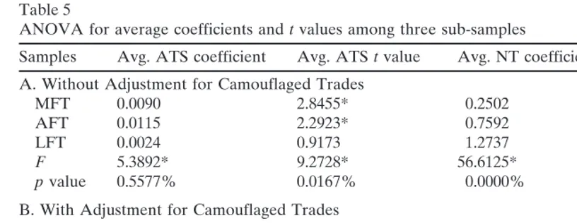
Both the ATS and NT coefficients are significantly different among the three

sub-samples since the p value for the ANOVA of ATS and NT coefficients are all less

than 1%. Overall, the less frequently traded stocks have lower ATS coefficients and higher NT coefficients. Table 5 reports the ANOVA of coefficients andtvalues among three sub-samples for two variables (ATS and NT). Results from the ANOVA also indicate that less frequently traded stocks have lower t values for ATS coefficients and highertvalues for NT coefficients.

(13)

GMM estimates of volatility regressions without an adjustment for camouflaged trades: A summary of three random samples

Median of Mean of

Panel A The Most Frequently Traded Stocks Mean (Median)R2₅_{28.21% (28.93%)}

Intercept 0.057 20.025 20.171 0.095 0.95

Average Trade Size 2.530* 2.845* 19.504* 0.009 6.3688*

Number of Trades 12.441* 12.232* 83.858* 0.2502 10.6017*

Monday Dummy 0.175 0.149 1.021 0.258 0.9416

Lag 1 Volatility 1.682** 1.662** 11.394* 0.0537 5.9513*

Panel B The Average Frequently Traded Stocks Mean (Median)R2₅_{35.01% (34.76%)}

Intercept 21.319 21.255 28.604* 20.2201 23.2949*

Number of Trades 16.401* 16.167* 110.835* 0.7592 13.5089*

Monday Dummy 20.096 0.08 0.548 0.0172 0.4468

Lag 1 Volatility 1.077 0.852 5.841* 0.0273 3.1645*

Panel C The Least Frequently Traded Stocks Mean (Median)R2₅_{35.09% (36.61%)}

Intercept 22.710* 22.564* 217.578* 20.3046 211.9451*

Average Trade Size 0.765 0.917 6.287* 0.0024 0.9711

Number of Trades 17.795* 17.232* 118.137* 1.274 12.6139*

First Half Hour Dummy 1.921** 2.187* 14.993* 0.6134 7.1409*

Monday Dummy 20.272 20.17 21.165 20.0233 20.759

Lag 1 Volatility 0.451 0.514 3.524* 0.0161 2.0201*

Estimates of the following regression for the three random sample (47 stocks each): VOLit5 ai1 giATSit1 biNTit1 hiOPENt1 viCLOSEt1 piMONDAYt1

o

14

n51

linVOLit2n1 mit

(14)

← →

in the number of transactions. Furthermore, return volatility exhibits significant varia-tions over the intraday periods. The volatility is significantly higher in the opening period.

The finding that average trade size has a significant effect on return volatility at the intraday level may not be surprising. Since volume is basically the aggregate of trades with different size, as the time interval gets shorter, the average trade size should contain more important information impounded in volume. In the limit, when the width of intervals approaches 0 (continuity), volume and average trade sizes are essentially equivalent. Hence, average trade size contains most of the information in volume at very short intervals. On the other hand, as the time interval gets wider, the average trade size effect could be washed out because of the aggregation, rendering more information to the frequency of trades. Thus, the empirical relation between return volatility and average trade size may depend on the time interval of data measurement.

4.2. Tests of the sensitivity to camouflaged trades

A familiar phenomenon in stock transactions, which may cause a problem for our empirical estimation, is that a large block trade may be divided into several smaller trades in the final transaction report. A rationale for this rearrangement of the trade report is to reduce the impact of large trades on market price. Alternatively, informed traders may camouflage their trading activities by strategically making several small-sized trades rather than one large trade. Such trading or reporting pattern may attenu-ate the relation between the size of trades and return volatility. For example, if a large order is divided into five smaller orders, the frequency of trades increases from one to five while the average trade size reduces to one fifth of the original level. Any price changes resulting from this trading would then appear to be associated more with trade frequency. As an order is divided into a greater number of smaller orders, the frequency of trades will become larger and average trade size smaller. In the extreme case where trade frequency is very large and average trade size is very small, price changes would be attributed to trade frequency alone.

To assess the potential effect of order splitting, we combined trades that exhibit this type of pattern using the following procedure. We first identified any trades that had a size larger than 1,000 shares and were reported less than 5 seconds apart. We then checked whether these trades had the same transaction price (traded at the same side) and were traded at the same quotes. We combined these trades into one trade when these conditions were met. This ad hoc data adjustment allows us to assess the potential effect of camouflaged trades on empirical estimation.

(15)

ANOVA for average coefficients andtvalues among three sub-samples

Samples Avg. ATS coefficient Avg. ATStvalue Avg. NT coefficient Avg. NTtvalue A. Without Adjustment for Camouflaged Trades

MFT 0.0090 2.8455* 0.2502 12.2320*

AFT 0.0115 2.2923* 0.7592 16.1665*

LFT 0.0024 0.9173 1.2737 17.2315*

F 5.3892* 9.2728* 56.6125* 17.3480*

pvalue 0.5577% 0.0167% 0.0000% 0.0000%

B. With Adjustment for Camouflaged Trades

MFT 0.0092 2.9474* 0.2533 12.0990*

AFT 0.0110 2.3124* 0.7451 16.0056*

LFT 0.0025 0.9292 1.2804* 17.2336**

F 4.7809* 9.8450* 56.9892 18.0655

pvalue 0.9828% 0.0101% 0.0000% 0.0000%

MFT is the most frequently traded stock sample, AFT is the average frequently traded stock sample, and LFT is the least frequently traded stock sample. A is based on the estimated results from Table 4 under the case without an adjustment for camouflaged trades, while B is based on the estimated results from Table 7 under the case with an adjustment for camouflaged trades. ATS stands for the average trade size, while NT is the number of trades at the 30-minute interval. TheFstatistics test the hypothesis that the coefficients (ortvalues) among three sub-samples are equal. * indicates a significance level of 5% or better for two-tailed test.

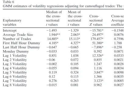
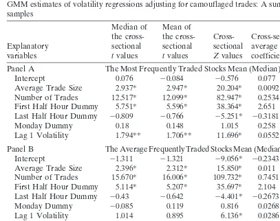
trade size rises to 2.312, while the meantvalue of trade frequency drops to 16.006. The results hence provide some evidence that trade camouflage may attenuate the volatility–volume relation. We hesitate to add that our data adjustment method is ad hoc and to some extent may underestimate the number of camouflaged trades. This identification problem may not be completely resolved until a better-coded data set is available. Nevertheless, our results reveal that order splitting can weaken the empirical relation between average trade size and return volatility.

4.3. Tests using log transaction variables

In principle, a better way to decompose the total volume effect would be to take a log transformation of the trade-related variables. Algebraically, total volume (V) is simply the product of average trade size (ATS) and the number of transaction (NT). With a log transformation, log volume (log V) is equal to the sum of log average trade size (log ATS) and log trade frequency (log NT). The log transformation thus yields a linearly separable decomposition for the total volume effect.

(16)

← →

Table 6

GMM estimates of volatility regressions adjusting for camouflaged trades: The full sample Median of Mean of

Explanatory sectional sectional sectional Average the average

Intercept 21.493 21.329 215.781* 20.1548 23.5916*

Number of Trades 14.885* 15.113* 179.457* 0.7596 14.4137*

Monday Dummy 20.033 0.033 0.392 0.0871 0.9396

Lag 1 Volatility 0.851 1.038 12.326* 0.0333 6.5881*

Lag 2 Volatility 20.06 0.072 0.855 0.0021 0.7794

Lag 3 Volatility 20.002 0.105 1.247 0.0028 0.9495

Lag 4 Volatility 20.055 0.094 1.116 0.0034 1.0948

Lag 5 Volatility 0.119 0.324 3.847* 0.0098 2.6361*

Lag 6 Volatility 0.12 0.115 1.366 0.0035 1.3511

Lag 7 Volatility 0.276 0.263 3.123* 0.0085 2.4245*

Lag 8 Volatility 20.015 0.081 0.962 0.0027 0.7664

Lag 9 Volatility 20.319 20.072 20.855 20.0022 20.788

Lag 10 Volatility 20.083 20.028 20.332 20.0005 20.1429

Lag 11 Volatility 0.234 0.257 3.052* 0.0074 2.5292*

Lag 12 Volatility 0.199 0.28 3.325* 0.0085 3.4431*

Lag 13 Volatility 20.204 0.033 0.392 0.001 0.3732

Lag 14 Volatility 20.188 20.041 20.487 20.0012 20.4312

Estimates of the following regression for the full random sample (141 stocks): VOLit5 ai1 giATSit1 biNTit1 hiOPENt1 viCLOSEt1 piMONDAYt1

o

14

n51

linVOLit2n1 mit

iat timet, OPENtis a dummy variable that is equal to 1 for the open half hour and 0 otherwise, CLOSEt is a dummy variable that is equal to 1 for the close half hour and 0 otherwise, MONDAYtis a dummy variable that is equal to 1 for Mondays and 0 otherwise, and the coefficientslinmeasure the persistence in volatility of securityi. The sample period is from April 1995 to June 1995. Each regression has 819 time series observations. * indicates a significance level of 5% or better for two-tailed test whereas ** indicates a significance level of 5% for one-tailed test. The cross-sectionalZvalue in the column 4 is calculated as the meantvalue multiplied by√141. The Tvalue in the last column is calculated as the cross-sectional average coefficient in column 5 divided by the standard error of the cross-sectional coefficient. Mean (Median)R2₅_{32.70% (32.17%).}

of missing values for the average frequently traded and least frequently traded stock samples. This may cause a problem of inefficiency in our empirical estimation. There-fore, we decide to report only the log results for most frequently traded stocks.

(17)

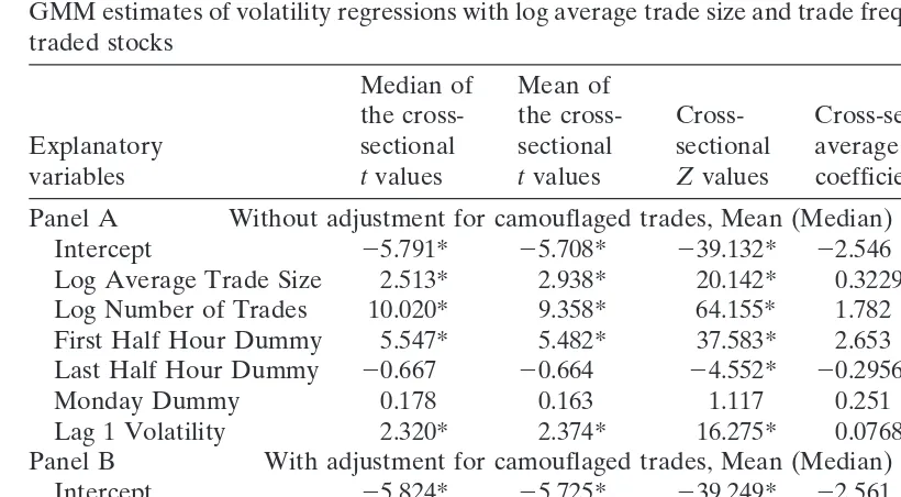
power of the log ATS. The average t statistic of average trade size increases from 2.845 to 2.938, while that of trade frequency decreases from 12.232 to 9.358. Table 8 B shows the results of GMM estimation for the data adjusted for camouflaged trades. The results indicate a further increase in the averagetvalue of average trade size (to 3.084) and a decrease in the average t value of frequency of trades (to 9.262). The aggregate T statistics for log ATS also increase slightly for both data sets with and without an order adjustment. The results indicate that log transformation seems to reduce the effect of trade frequency more than to bring up the explanatory power of average trade size. Overall, the results reinforce our preceding conclusion that average trade size contains nontrivial trade information.

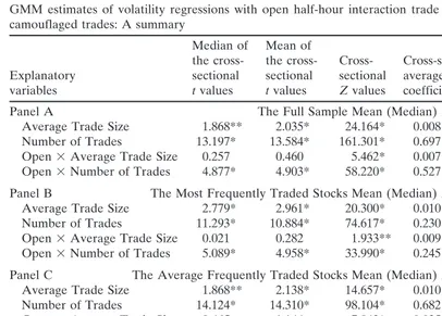
4.4. The volatility–volume relation at the market opening

To examine whether the relation between return volatility and the size and frequency of trades varies over intraday periods, we estimate an equation [Eq. (2a)] that incorpo-rates slope dummies to allow the coefficients of trade-related variables in the opening period to be different from those of the remaining trading periods. Although estimates were obtained for all data samples, in the interest of brevity we only report the results for the data adjusted for camouflaged trades in Table 9. The results for the data without an adjustment for camouflage trades are very similar to those with an adjustment. Also, to provide a more concise summary, we highlight only the estimation results for the trade-related variables.

The overall results show that the effect of the frequency of trades (NT) on return volatility is much higher in the opening period. The coefficients of the slope dummy variables (OPEN3NT) are all significant at the 1% level for the full sample as well as for the three frequency groups. On the other hand, the effect of average trade size does not appear to be significantly different in the opening period.

(18)

← →

Table 7

GMM estimates of volatility regressions adjusting for camouflaged trades: A summary of three random samples

Median of Mean of

Panel A The Most Frequently Traded Stocks Mean (Median)R2₅_{28.02% (28.99%)}

Intercept 0.076 20.084 20.576 0.077 0.77

Number of Trades 12.517* 12.099* 82.947* 0.2534 10.5583*

Monday Dummy 0.18 0.148 1.015 0.258 0.9416

Lag 1 Volatility 1.794** 1.706** 11.696* 0.0552 6.1368*

Panel B The Average Frequently Traded Stocks Mean (Median)R2₅_{34.96% (34.29%)}

Intercept 21.311 21.321 29.056* 20.2343 23.5286*

Number of Trades 15.670* 16.006* 109.732* 0.7451 13.6967*

Monday Dummy 20.085 0.119 0.816 0.0268 0.6961

Lag 1 Volatility 1.014 0.895 6.136* 0.0286 3.3863*

Panel C The Least Frequently Traded Stocks Mean (Median)R2₅_{35.12% (35.83%)}

Intercept 22.711* 22.582* 17.701* 20.3073 211.9109*

Number of Trades 17.809* 17.234* 118.150* 1.28 12.5490*

First Half Hour Dummy 1.904** 2.177* 14.925* 0.6091 7.0908*

Monday Dummy 20.272 20.169 21.159 20.0235 20.768

Lag 1 Volatility 0.451 0.514 3.524* 0.0161 2.0201*

Estimates of the following regression for the three random samples (47 stocks each): VOLit5 ai1 giATSit1 biNTit1 hiOPENt1 viCLOSEt1 piMONDAYt1

o

14

n51

linVOLit2n1 mit

(19)

GMM estimates of volatility regressions with log average trade size and trade frequency: Most frequently traded stocks

Median of Mean of

Panel A Without adjustment for camouflaged trades, Mean (Median)R2₅_{25.44% (25.89%)}

Intercept 25.791* 25.708* 239.132* 22.546 28.8711*

Log Average Trade Size 2.513* 2.938* 20.142* 0.3229 7.5798*

Log Number of Trades 10.020* 9.358* 64.155* 1.782 15.6316*

Monday Dummy 0.178 0.163 1.117 0.251 0.9161

Lag 1 Volatility 2.320* 2.374* 16.275* 0.0768 8.5183*

Panel B With adjustment for camouflaged trades, Mean (Median)R2₅_{25.36% (25.73%)}

Intercept 25.824* 25.725* 239.249* 22.561 28.8924*

Log Average Trade Size 9.956* 9.262* 63.497* 1.772 15.5439*

Log Number of Trades 5.487* 5.479* 37.562* 2.653 6.3469*

First Half Hour Dummy 20.687 20.662 24.538* 20.2954 24.2020*

Last Half Hour Dummy 0.201 0.162 1.111 0.251 0.9161

Monday Dummy 2.304* 2.397* 16.433* 0.0775 8.6410*

Lag 1 Volatility 20.127 0.043 0.295 0.0013 0.2746

Estimates of the following regression for the most frequently traded stock sample (47 stocks): VOLit5 ai1 giLATSit1 biLNTit1 hiOPENt1 viCLOSEt1 piMONDAYt1

o

14

n51

linVOLit2n1 mit

t, LATSitis the average trade size (total share volume divided by the number of transactions) for security

iat timet, OPENtis a dummy variable that is equal to 1 for the open half hour and 0 otherwise, CLOSEt is a dummy variable that is equal to 1 for the close half hour and 0 otherwise, MONDAYtis a dummy variable that is equal to 1 for Mondays and 0 otherwise, and the coefficientslinmeasure the persistence in volatility of securityi. The sample period is from April 1995 to June 1995. Each regression has 819 time series observations. * indicates a significance level of 5% or better for two-tailed test whereas ** indicates a significance level of 5% for one-tailed test. The cross-sectionalZvalue in the column 4 is calculated as the meantvalue multiplied by√47. The Tvalue in the last column is calculated as the cross-sectional average coefficient in column 5 divided by the standard error of the cross-sectional coefficient.

appears that only the opening period exhibits a distinct relation between the return volatility and trade frequency.

5. Summary

(20)

← →

Table 9

GMM estimates of volatility regressions with open half-hour interaction trade variables adjusting for camouflaged trades: A summary

Median of Mean of

Panel A The Full Sample Mean (Median)R2₅_{30.92% (30.92%)}

Number of Trades 13.197* 13.584* 161.301* 0.697 14.1667*

Open3Average Trade Size 0.257 0.460 5.462* 0.007 1.511

Open3Number of Trades 4.877* 4.903* 58.220* 0.527 9.9962*

Panel B The Most Frequently Traded Stocks Mean (Median)R2₅_{26.01% (27.25%)}

Number of Trades 11.293* 10.884* 74.617* 0.230 10.8396*

Open3Average Trade Size 0.021 0.282 1.933** 0.009 1.9431**

Panel C The Average Frequently Traded Stocks Mean (Median)R2₅_{31.75% (32.23%)}

Number of Trades 14.124* 14.310* 98.104* 0.682 12.8120*

Open3Average Trade Size 0.465 1.144 7.843* 0.025 2.5302*

Panel D The Least Frequently Traded Stocks Mean (Median)R2₅_{35.01% (35.20%)}

Number of Trades 16.379* 15.560* 106.674* 1.180 12.4572*

Open3Average Trade Size 20.967 20.046 20.315 20.011 21.225

Estimates of the following regression:

(21)

for correlations among the residuals of individual securities to obtain more efficient estimates. Empirical results show that stock return volatility has a significant positive relation to both average trade size and the number of transactions. The coefficients of average trade size are more significant for stocks that are actively traded. Further-more, the effect of trade frequency on return volatility is much higher in the opening period, whereas the effect of average trade size is not.

We also examine the potential impact of camouflaged trades using a simple adjust-ment method. We find that camouflaged trades tend to attenuate the relation between volatility and average trade size. In addition, using a log transformation to decompose the total volume effect, we find that the explanatory power of trade frequency drops substantially for more frequently traded stocks.

Contrary to JKL’s finding, our results indicate that average trade size has significant information content for stock prices. However, while both the frequency and size of trades contain nontrivial information, the results continue to show that the frequency of trades has higher explanatory power for return volatility than average trade size does even at the intraday intervals. The results thus suggest a need to develop market microstructure models that endogenize both the size and frequency of trades.

Notes

1. The contemporaneous positive relation between volume and absolute return has been strongly supported by studies using both intraday (e.g., Wood et al., 1985; Jain and Joh, 1988) and daily data (e.g., Clark, 1973; Tauchen & Pitts, 1983; Harris, 1986).

2. Trading volume is equal to the average trade size times the frequency of trades in a time interval.

3. This method was originally proposed by Schwert (1989). 4. Eq. (1) is basically the same as:

Rit 5vi1

o

5

k52

aikWkt1

o

14

n51

binRit2n1eit

where virepresents the fixed effect on Monday for each security.

5. As explained later, we also incorporated time-of-day dummies for other trading hours. However, none of these dummy variables were significant.

6. See Jones, Kaul, and Lipson (1994).

7. See Lo and MacKinlay (1990) for the evidence of serial and cross-serial correla-tions among stock returns.

8. In Eq. (2), there are 19 regressors and 1 constant term.

9. The original sample includes 150 stocks. Nine stocks were removed because of data problems. To be included in the sample, a stock must have at least one trade in any of the trading days over the sample period.

10. The results of the first-stage return model are available upon request.

(22)

← →

the cross-sectional meantvalue multiplied by the squared root ofN, whereN is the number of firms in the sample.

12. T is equal to the mean of the coefficients of individual stocks divided by the standard error of the mean coefficient.

References

Anderson, T. G. (1996). Return volatility and trading volume: an information flow interpretation of stochastic volatility.Journal of Finance 50, 169–204.

Admati, A. R., & Pfleiderer, P. (1988). A theory of intraday trading patterns: volume and price variability.

Review of Financial Studies 1, 3–40.

Blume, L., Easley, D., & O’Hara, M. (1994). Market statistics and technical analysis: the role of volume.

Journal of Finance 49, 153–181.

Campbell, J., Lo, A.W., & MacKinlay, A. C. (1997).The Econometrics of Financial Markets.Princeton, NJ: Princeton University Press.

Clark, P. K. (1973). A Subordinated stochastic process model with finite variance for speculative prices.

Econometrica 41, 135–155.

Easley, D., Kiefer, N. M., O’Hara, M., & Paperman, J. B. (1996). Liquidity, information, and infrequently traded stocks.Journal of Finance 51, 1405–1436.

Foster, F. D., & Viswanathan, S. (1990). A theory of interday variations in volume, variance, and trading costs in securities markets.Review of Financial Studies 3, 593–624.

Foster, F. D., & Viswanathan, S. (1993). Variations in trading volume, return volatility, and trading costs: evidence on recent price formation models.Journal of Finance 48, 187–211.

Gallant, A. R., Rossi, P. E., & Tauchen, G. E. (1992). Stock prices and volume.Review of Financial

Studies 5, 199–242.

Grundy, B. D., & McNichols, M. (1989). Trade and revelation of information through prices and direct disclosure.Review of Financial Studies 2, 495–526.

Hansen, L. P. (1982). The large properties of generalized method of moments estimators.Econometrica 50, 1029–1054.

Harris, L. (1986). Cross-security tests of the mixture of distribution hypothesis.Journal of Financial and

Quantitative Analysis 21, 39–46.

Holden, C. W., & Subrahmanyam, A. (1992). Long-lived private information and imperfect competition.

Journal of Finance 47, 247–270.

Holthausen, R. W., & Verrecchia, R. E. (1990). The effects of informedness and consensus on price and volume behavior.Accounting Review 65, 191–208.

Jain, P. C., & Joh, G. (1988). The dependence between hourly price and trading volume.Journal of

Financial and Quantitative Analysis 23, 269–283.

Jones, M. J., Kaul, G., & Lipson, M. L. (1994). Transactions, volume, and volatility.Review of Financial

Studies 7, 631–651.

Karpoff, J. M. (1987). The relation between price changes and trading volume: a survey. Journal of

Financial and Quantitative Analysis 22, 109–126.

Kim, O., & Verrecchia, R. E. (1991). Market reaction to anticipated announcements.Journal of Financial

Economics 30, 273–309.

Kyle, A. S. (1985). Continuous auctions and insider trading.Econometrica 53, 1315–1335.

Lamoureux, C. G., & Lastrapes, W. D. (1990). Heteroskedasticity in stock return data: volume vs. GARCH effects.Journal of Finance 45, 221–229.

Lo, W. A., & MacKinlay, A. C. (1990). When are contrarian profits due to stock market overreaction?

Review of Financial Studies 3, 175–205.

(23)

X.E. Xu, C. Wu / International Review of Economics and Finance 8 (1999) 375–397 397 Schwert, G. W. (1989). Why does stock market volatility change over time?Journal of Finance 44,

1115–1153.

Stoll, H. R., & Whaley, R. (1990). Stock market microstructure and volatility.Review of Financial Studies 3, 31–71.

Tauchen, G. E., & Pitts, M. (1983). The price volatility-volume relationship on speculative markets.

Econometrica 51, 485–505.

Wood, R., McInish, T., & Ord, J. (1985). An investigation of transaction data for NYSE stocks.Journal