www.elsevier.comrlocatereconbase
Three analyses of the firm size premium
Joel L. Horowitz
a, Tim Loughran
b, N.E. Savin
a,) aHenry B. Tippie College of Business, Department of Economics, 108 John Pappajohn Business Building, The UniÕersity of Iowa, Iowa City, IA 52242-1000, USA
b
UniÕersity of Notre Dame, P.O. Box 399, Notre Dame, IN 46556-0399, USA
Accepted 11 March 2000
Abstract
The size premium for smaller companies is one of the best-known academic market anomalies. The relevant issue for investors is whether size premium for small-cap stocks is still positive, and, if so, whether its magnitude is substantial. In our analysis, we use annual compounded returns, monthly cross-sectional regressions, and linear spline regressions to investigate the relation between expected returns and firm size during 1980–1996. All three methodologies report no consistent relationship between size and realized returns. Hence, our results show that the widespread use of size in asset pricing is unwarranted. q2000
Elsevier Science B.V. All rights reserved.
JEL classification: G12; G14
Keywords: Size premia; Asset pricing; Spline regressions
1. Introduction
The size premium for smaller companies is one of the best-known academic
Ž . Ž .
market anomalies. Reinganum 1981 and Banz 1981 reported that for U.S. stock market data prior to 1980 small-cap stocks had substantially higher returns compared to large-cap stocks. This evidence played an important role in the
)Corresponding author. Fax:q1-319-335-195.
Ž .
E-mail address: [email protected] N.E. Savin .
0927-5398r00r$- see front matter q2000 Elsevier Science B.V. All rights reserved.
Ž .
development of small-cap mutual funds designed to take advantage of the size premium. Further, it quickly created a cottage industry for academics to explain
Ž
the reasons for the anomaly’s existence see Barry and Brown, 1984; Brown et al., 1983; Keim 1983, 1989; Schultz, 1983; Stoll and Whaley, 1983; Reinganum,
. 1983 .
The relevant issue for investors is whether size premium for small cap stocks is still positive, and, if so, whether its magnitude is substantial. Recent studies by
Ž . Ž .
Dimson and Marsh 1999 and Horowitz et al. 1999 suggest that this market anomaly may have disappeared, and, perhaps, that the size premium may have gone into reverse. Indeed, on the basis of these studies, large-cap firms appear to have higher returns than small cap firms do. A skeptic’s view of the size effect may be that it never really existed. Academic predictions often fail in
out-of-sam-Ž .
ple tests. As an example, Goyal and Welch 1999 show that the lagged dividend yield has no ability to predict out-of-sample equity premia. This contradicts the
Ž .
evidence presented by Fama and French 1988 and others on the predicative ability of the lagged dividend yield.
In this paper we investigate whether there is a size effect for the period 1980–1996 using three different methodologies. The size effect refers to the relation between the expected return and firm size. We interpret this relation as a population regression function. We investigate the relation between expected
Ž .
return and firm size for data from the New York Stock Exchange NYSE ,
Ž .
American Stock Exchange Amex , and NASDAQ during 1980–1996. Following the conventional methodology, firms are sorted into NYSE-based size deciles where size is defined as the market value of equity from the last trading day of the prior year.
Our three analyses to examine the size effect are annual compound returns, monthly cross-sectional regressions and linear spline regressions during 1980– 1996. We report annual compounded returns as well as the average regression
Ž .
slopes from the Fama and MacBeth 1973 monthly cross-sectional regressions during the 204-month sample period. Both the annual compounded returns and
Ž .
average slope coefficients from the Fama and MacBeth 1973 monthly regres-sions indicate a somewhat flat relationship between market capitalization and realized returns.
The linear spline, which is a continuous piecewise linear function, is also used to approximate the population regression function. The spline is a natural approxi-mation for the size effect regression since in finance the convention is to group the firms for the purpose of analysis. The estimated spline regression varies substan-tially from year-to-year about a basically flat population regression line. Hence, our evidence based on traditional methods that the size premium has vanished since 1980 is consistent with the evidence produced by the spline analysis
2. Data
The data used in the our paper consists of all NYSE, Amex, and NASDAQ Ž
operating firms American Depository Receipts, closed-end funds, and real estate .
investment trusts are excluded listed on the University of Chicago Center for
Ž .
Research in Security Prices CRSP daily tapes on the last day of a calendar year during 1979–1995. The aggregate sample includes over 98,000 firm years.
Ž .
Monthly stock returns dividends plus capital gainsrlosses are constructed by
compounding the daily returns within the month. No survivor bias is present in our
Ž .
analysis. Firms that are delisted from the CRSP tapes for good i.e., takeovers and
Ž .
bad i.e., bankruptcies reasons are included in the results until their particular delisting date.
Following the practice in finance, the decile cutoffs are determined each year Ž
by ranking all NYSE firms on the basis of market value shares outstanding times
. Ž
share price determined on the last day of the prior calendar year December 31 of .
year ty1 . The market value cutoffs are calculated by having an equal number of
NYSE firms within each size decile for each calendar year. The majority of firms are in the smallest size decile because most NASDAQ and Amex firms have smaller market values than the typical NYSE firm.
Ž We have departed from the sample procedure used by Fama and French 1992,
.
1993 . Their procedure requires sample firms to be listed on both the CRSP and Compustat tapes when jointly testing for size and book-to-market effects. As a consequence, some have argued that their empirical results are subject to a
Ž .
survivor bias. For example, Kothari et al. 1995 claim that this data requirement causes the results of Fama and French to be overstated because of Compustat’s well known tendency to back-fill the accounting data of small firms which subsequently were extreme winners. Our results are unaffected by any potential survivor bias since we do not require the use of Compustat data.
3. Empirical results
Table 1 reports the annual compounded returns categorized by NYSE-de-termined size deciles during our sample period. NYSE, Amex, and NASDAQ firms in the smallest decile have annual compounded returns of approximately 15% compared to 14.4% for size decile 5, and slightly over 16% for firms in the largest size decile. The lowest annual compounded return occurs in size decile 2. Size decile 7 reports the highest annual compounded return of 16.7%. Overall, there appears to be a reverse size effect pattern. That is, large firms have slightly higher realized annual compounded returns than small firms do.
Ž Following the linear regression methodology used by Fama and French 1992,
. Ž .
regres-Table 1
Annual compounded returns by size deciles, 1980–1996
The sample includes all NYSE, Amex, and NASDAQ operating firms listed on the CRSP daily tape during 1980–1996. Size decile cutoffs are determined each year by ranking all NYSE firms on the
Ž .
basis of market value shares outstanding times share price determined on the last day of the prior
Ž . Ž
calendar year i.e., December 31 of year ty1 . Returns include all distributions i.e., both capital and
. Ž
dividend gains . The sample covers the time period from January 1980 through December 1996 204
.
months .
Ž .
NYSE size decile Annual return %
Smallest 14.99
sions. Our dependent variable is the raw monthly return for stock i. The independent variable is the natural logarithm of firm size as of December 31 of the prior calendar year.
In our paper, the average parameter value for the natural logarithm of market
Ž .
value of equity isy0.09 t-statistic ofy1.49 . The corresponding numbers from
Ž . Ž .
Fama and French 1992, Table III are y0.11 t-statistic of y1.99 . In both
papers, the t-statistics are created by dividing the average slope by its time-series
Ž .
standard error. Since the average slope on ln size is not statistically different from
Table 2
Average slopes from monthly regressions of percentage stock returns on the logarithm of market capitalization, 1980–1996
Ž .
ri jsa0 jqa1 jln sizei jqe .i j
The sample includes all NYSE, Amex, and NASDAQ operating firms listed on the CRSP daily tape
Ž .
during 1980–1996. Monthly returns include all distributions i.e., both capital and dividend gains . The
Ž .
sample covers the time period from January 1980 through December 1996 204 months . ri j is the
Ž .
percentage return on stock i in calendar month j. ln sizei jis the natural logarithm of the market value
Ž .
of equity stock price multiplied by shares outstanding of firm i as of December 31 of the prior year.
Ž .
The values of ln size are winsorized at the respective 1% and 99% levels. The parameter values are the average of the cross-sectional regressions. The t-statistics are in parenthesis and are determined by dividing the average coefficient by its time-series standard error.
Item Intercept Natural logarithm of
market capitalization
Ž . Ž .
zero, no size effect appears to exist using this linear regression methodology during 1980–1996. This evidence of no size effect is also consistent with the annual compounded return pattern reported in Table 1.
Our last methodology is the linear spline regression. The basic idea is that any continuous function can be approximated arbitrarily well by a piecewise linear function, that is, a continuous function composed of straight lines. One linear
segment represents the function for size values below s . Another linear segment1
represents the function for values between s1 and s , and so on. The linear2
segments are arranged so that they join at s , s , . . . , which are called knots. In1 2
our application the knots are determined by the size deciles, or more precisely, by the endpoints of the size intervals. For a brief examination of the linear spline, see
Ž .
Greene 1993, pp. 235–238 . A more detailed treatment is found in Seber and
Ž .
Wild 1989, pp. 481–489 .
To graphically display the spline regressions, we need identical yearly decile cutoffs, that is, only one set of decile cutoffs for all years. Thus, to enhance comparisons, we created decile cutoffs by grouping all NYSE firms together
Žbased on 1996 dollars . After combining all NYSE firms from all years together,.
a single set of decile cutoffs was created. Although this procedure has a look-ahead bias, our spline regression results are unaltered if we instead placed firms into yearly determined size deciles.
The spline analysis was carried out for the full year and January sub-periods. For firms delisted from the exchanges during the calendar year, we splice in, on a point-forward basis, the value-weighted NYSE–Amex–NASDAQ Index. Hence, all regressions have the same number of observations for a given cohort year. The February to December spline graphs look very similar to the full year, thus are not reported. The results of the analysis are presented in two types of graphs. One
Ž .
presents the estimated expected predicted return as a function of size, and due to their appearance, they are referred to as spaghetti graphs. The other graph presents the estimated slopes within each decile, and we refer to these as bubble graphs.
Ž .
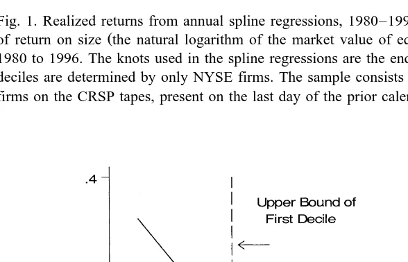
Figs. 1 and 2 spaghetti graphs show the estimated expected returns as a function of firm size. Fig. 1 is for the full year while Fig. 2 is for January. In the
Ž .
figures, the size scale log of market capitalization in millions of dollars on the
x-axis roughly varies from 2 to 11. This corresponds to a variation in market
capitalization from approximately $7 million to $60 billion in 1996 dollars. To lessen the impact of extreme outliers, firms with market values greater than the top 1% of all NYSE firms are truncated at the 1% level. Firms below the bottom 99 percentile of NYSE market values are given the market value of the 99 percentile. The dotted vertical line represents the upper bound of the first decile. The cutoff for the first decile is approximately 4.2, which corresponds to approximately $70 million.
Fig. 1. Realized returns from annual spline regressions, 1980–1996. The 17 annual spline regressions
Ž .
of return on size the natural logarithm of the market value of equity were estimated for each year, 1980 to 1996. The knots used in the spline regressions are the endpoints of the size deciles where the deciles are determined by only NYSE firms. The sample consists of all NYSE, Amex, and NASDAQ firms on the CRSP tapes, present on the last day of the prior calendar year.
Fig. 2. Realized returns from January spline regressions, 1980–1996. The 17 January spline regressions
Ž .
relation across the years. Even the signs of the slopes for a given decile vary across the years. The most striking feature of the spaghetti graphs is that after the first decile the slopes are often positive. Notice, for example, that in the second decile, the slopes are overwhelmingly positive.
Ž .
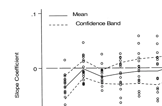
This observation is explored further in Figs. 3 and 4 bubble graphs . Again,
Ž .
Fig. 3 is for the full year while Fig. 4 is for January only. Fama and French 1992 also focused on the estimated monthly slopes. However, they ran a least squares regression of return on size for every month and took the average of the least
Ž .
squares slopes. Following the spirit of Fama and French 1992 , the bubble graphs treat the slope of the relation between size and returns as a random variable. Each year provides a new draw of the slope function. One can then ask whether the average slope is negative or positive. The bubbles in the graphs show the estimated slopes for each of the 17 years and 10 size groups. The solid lines show the average estimated slopes, and the long-dash lines indicate the location of a slope of zero. The dotted lines indicate a joint confidence band for the slopes of the true but unknown mean.
The interpretation of these bands is that, subject to the approximation described below, they contain the true but unknown means with a probability that is at least
Ž .
95%. In Fig. 3 full year , the confidence band excludes zero only in the second
Fig. 3. Slope coefficients from annual spline regressions, 1980–1996. The 17 annual spline regressions
Ž .
of return on size the natural logarithm of the market value of equity were estimated for each year,
Ž .
Fig. 4. Slope coefficients from January spline regressions, 1980–1996. The 17 January spline
Ž .
regressions of return on size the natural logarithm of the market value of equity were estimated for each year, 1980 to 1996. For each year, the estimated slope for each size decile is represented by a
Ž .
circle bubble . The size deciles are determined by only NYSE firms. The sample consists of all NYSE, Amex, and NASDAQ firms on the CRSP tapes, present on the last day of the prior calendar year. The sample mean of the estimated slopes within each decile is represented by a solid line. The 95% Bonferroni is represented by the dashed line.
decile. Furthermore, the average of the decile slopes is essentially zero in all but
Ž .
the second decile where it is positive. In Fig. 4 January only , the confidence band excludes zero only in the first and third deciles. Thus, there is an observed size effect in January for our sample of firms. In these deciles, the mean slope is negative, although it can be seen that the slopes of individual years are not always negative. In the remaining deciles, there is no basis for concluding that the mean slope of the relation between size and return is different from zero.
Clearly if our sample period contains too many bearish years, the lack of a consistent size effect would not be surprising. This is because small firms have, on
Ž .
average, higher betas than large firms see Fama and French, 1992 . However, the 1980–1996 period was a strong bull market. Using the CRSP valued-weighted
NYSErAmexrNASDAQ Index as the market return, 14 calendar years out of our
The confidence bands assume that the sample mean of the estimated slopes is approximately normally distributed. The central limit theorem insures that this is an accurate approximation if the sample size is sufficiently large. In small samples
Žsuch as ours, where the size is 17 , the approximation is likely to produce.
confidence bands that are too narrow. In other words, AexactB bands would be
wider and, therefore, more likely to contain zero. In addition, the bands are also based on the Bonferroni inequality, so they have a coverage probability that is at least 95%, but not exactly 95%. The Bonferroni inequality is a way of obtaining joint confidence intervals for parameters whose estimates are not independent of
Ž .
one another i.e., our mean slopes .
In addition, we estimated the pooled regression using a generalized least squares procedure to account for the heteroscedasticity of the returns. For this purpose, we estimated the standard deviation of the returns within each decile
Ž .
using the pooled data and then divided the regressors including the intercept by the estimated standard deviations. The spline regressions with the transformed
Ž .
variables were re-estimated by least squares with no intercept . The results were qualitatively similar to those obtained by ordinary least squares with the exception of the full year regression. For this regression, the estimated slope for the ninth decile was negative and significantly different from zero.
4. Conclusion
Ž
This paper examines whether the widespread use of size shares outstanding .
multiplied by stock price in asset pricing is justified by the empirically observed data. The analysis is based on data from the NYSE, Amex, and NASDAQ during 1980–1996. The evidence produced by the annual compounded returns and the
Ž .
Fama and MacBeth 1973 monthly regressions shows no systematic relation between expected return and size return. This is also consistent with the evidence from the spline regressions. In other words, the population regression function of expected return given size is essentially flat.
Ž . Ž .
Fama and French 1992 and Berk 1995 argue that small firms have higher risk that is compensated with higher long-run returns. This argument has two components. The first is empirical: small firms have higher average long-run returns. The second is theoretical: these higher returns are equilibrium compensa-tion for risk bearing. The weakness in their argument is the empirical component. There is no compelling evidence during the 1980–1996 period that small firms had higher realized returns. None of our three methodologies find evidence that small firms have higher realized returns than large firms do. Therefore, the agency
Ž .
arguments for the size effect, as proposed in Maug and Naik 1996 , are probably not valid. Our findings weaken any ex-post rationalization of the size effect.
realized returns will always be related to market value. On the other hand, the fact that the empirical evidence for 17 years has not supported the size effect should give one pause. Furthermore, money managers should not place bets on the size effect or any other market anomaly that cannot reliably be shown to work. It appears that the size effect is a typical academic discovery, strong in-sample evidence, weak out-of-sample results.
Acknowledgements
We would like to thank Utpal Bhattacharya, Franz Palm, Michael Stutzer, and two anonymous referees. The research of Joel L. Horowitz was supported in part by NSF grant SBR 9617925.
References
Banz, R.W., 1981. The relationship between return and market value of common stocks. Journal of Financial Economics 9, 3–18.
Barry, C.B., Brown, S.J., 1984. Differential information and the small firm effect. Journal of Financial Economics 13, 283–294.
Berk, J.R., 1995. A critique of size-related anomalies. Review of Financial Studies 8, 275–286. Brown, P., Kleidon, A., Marsh, T., 1983. New evidence on the nature of size-related anomalies in stock
prices. Journal of Financial Economics 12, 33–56.
Dimson, E., Marsh, P., 1999. Murphy’s law and market anomalies. Journal of Portfolio, 53–69. Fama, E.F., French, K.R., 1988. Dividend yields and expected stock returns. Journal of Financial
Economics 22, 3–25.
Fama, E.F., French, K.R., 1992. The cross-section of expected stock returns. Journal of Finance 47, 427–465.
Fama, E.F., French, K.R., 1993. Common risk factors in the returns on stocks and bonds. Journal of Financial Economics 33, 3–56.
Fama, E.F., MacBeth, J., 1973. Risk return and equilibrium: empirical tests. Journal of Political Economy 81, 607–636.
Goyal, A., Welch, I., 1999. Predicting the equity premium. UCLA working paper. Greene, W.H., 1993. Econometric Analysis. Macmillan, New York.
Horowitz, J.L., Loughran, T., Savin, N.E., 1999. The disappearing size effect. Research in Economics, in press.
Keim, D.B., 1983. Size related anomalies and stock return seasonality: empirical evidence. Journal of Financial Economics 12, 13–32.
Keim, D.B., 1989. Trading patterns, bid–ask spreads, and estimated security returns. Journal of Financial Economics 25, 75–97.
Kothari, S.P., Shanken, J., Sloan, R.G., 1995. Another look at the cross-section of expected stock returns. Journal of Finance 50, 185–224.
Maug, E., Naik, N. 1996. Herding and delegated portfolio management: the impact of relative performance evaluation on asset allocation. London Business School working paper.
Reinganum, M.R., 1983. The anomalous stock market behavior of small firms in January: some empirical tests for the tax-loss selling effects. Journal of Financial Economics 12, 89–104. Schultz, P., 1983. Transaction costs and the small firm effect: a comment. Journal of Financial
Economics 12, 81–88.
Seber, G.A.F, Wild, C.J., 1989. Nonlinear Regression. Wiley, New York.