Identifying Failing Companies: A
Re-evaluation of the Logit, Probit and
DA Approaches
Clive Lennox
This paper examines the causes of bankruptcy for a sample of 949 UK listed companies between 1987–1994. The most important determinants of bankruptcy are profitability, leverage, cashflow, company size, industry sector and the economic cycle. Tests for heteroskedasticity revealed that cashflow and leverage have significant non-linear effects, and taking account of these non-linearities improves the model’s explanatory power. In contrast to previous studies, the paper argues that well-specified logit and probit models can identify failing companies more accurately than discriminant analysis (DA). © 1999 Elsevier Science Inc.
Keywords: Bankruptcy; Discriminant analysis; Probit; Logit
JEL classification: C25, G33
I. Introduction
There have been numerous bankruptcy studies since the pioneering research of Beaver (1966) and Altman (1968). The contribution of this paper to the literature is two-fold. First, it evaluates the merits of using well-specified probit and logit models rather than discriminant analysis (DA). The earliest bankruptcy studies used DA to identify failing companies [Altman (1968); Altman et al. (1977); Beaver (1966); Blum (1974); Deakin (1972); Elam (1975); Norton and Smith (1979); Wilcox (1973)]. More recently, research-ers have used probit and logit methods, which require less restrictive assumptions [Ohlson (1980); Zmijewski (1984); Koh (1991); Hopwood et al. (1994); Platt et al. (1994)]. Despite this, previous studies have argued that, in practice, the explanatory power of probit and logit models is similar to that of DA [Press and Wilson (1978); Lo (1986);
Economics Department, Bristol University, Bristol, England.
Address correspondence to: Dr. C. Lennox, University of Bristol, Department of Economics, 8 Woodland Road, Bristol BS8 1TN, England.
Collins and Green (1982)]. However, it remains unclear whether there are potential gains from using probit and logit rather than DA, as previous probit and logit studies have not reported tests for misspecification. This is rather surprising, because Lagrange Multiplier (LM) tests for omitted variable bias and heteroskedasticity are easily calculated [Davidson and MacKinnon (1984)]. Tests for heteroskedasticity are particularly important because heteroskedasticity causes bias in both the coefficient estimates and their standard errors in probit and logit models [Yatchew and Griliches (1985)].1This paper appears to be the first bankruptcy study to report tests for omitted variable bias and heteroskedasticity.
Secondly, this study analyzes the effects of industry sector, company size, and the economic cycle on the probability of bankruptcy. Previous bankruptcy studies have mostly adopted a matched pairs technique for drawing samples of failing and non-failing companies. A sample of non-bankrupt companies is usually drawn by matching against the characteristics of bankrupt companies. These characteristics are generally chosen to be company size, industry sector, and year of failure. The advantage of the matching procedure is that it helps to cut the cost of data collection, as the proportion of failing companies in the population is very small.2One disadvantage with the matching approach is that it is not possible to investigate the effects of industry sector, company size or year of failure on the probability of bankruptcy [Jones (1987)]. In addition, the use of relatively small samples could lead to over-fitting. This study avoided these problems by collecting data on a large number of companies over an eight-year period, and by evaluating the effects of company size, industry sector, and the economic cycle on the probability of bankruptcy.
The structure of the rest of this paper is as follows. Section II outlines an economic theory of bankruptcy, and describes the tests for misspecification in probit and logit models. Section III explains the sample-selection method and describes the data. Section IV discusses the estimation results, and Section V compares predictive accuracy of the DA, probit and logit models. Section VI offers conclusions.
II. Theoretical Developments and Statistical Methodology
Previous empirical research has found that a company is more likely to fail if it is unprofitable, highly leveraged, and suffers cashflow difficulties [Altman (1986)]. Myers (1977) has outlined a theoretical model which helps to explain these findings. The model predicts that investors will choose to liquidate if the company’s liquidation value exceeds its going-concern value.3If profitable companies have higher going concern value, one should find that profitable companies are less likely to go bankrupt than unprofitable companies.
1In contrast, heteroskedasticity in regression models does not affect the consistency of coefficient estimates. 2In DA and logit estimation, a sample selection rule which results in the sample proportion being different
from the population proportion of failing companies merely biases the constant term [Lachenbruch (1975); Anderson (1972)]. In contrast, probit estimation requires the likelihood function to be weighted so that the sample proportion of bankrupt companies is approximately equal to the population proportion—otherwise all coefficient estimates are biased.
3Variations on this theme have been proposed following this research. In Bulow and Shoven (1978),
If contracting were complete, a company’s owners would contract with the manager to liquidate when the company’s liquidation value exceeds its going-concern value. When contracting is incomplete, financial structure can substitute for contracts [Aghion and Bolton (1992)]. In particular, managers may issue debt so that the company enters liquidation when it defaults on debt servicing. In this way, managers are able to signal that they are willing to act in the investors’ interests [Hart (1995)]. This implies that a company is more likely to enter bankruptcy when leverage is high.
Bankruptcy is usually triggered by default on debt servicing, and this is less likely to occur if the company has access to internal or external finance. A company with healthy cashflow has relatively easy access to internal finance, and so it is less likely to go bankrupt than a company with cashflow problems. Large companies are less likely to encounter credit constraints in the market for external finance because of reputation effects. Therefore, company size may be an important determinant of bankruptcy. Finally, the economic cycle and industry sector may determine a company’s access to finance.
Although early bankruptcy studies used DA to identify failing companies, its suitability rests on two assumptions. First, the explanatory variables are assumed to have a multi-variate normal distribution. Nevertheless, it is well known that the variables typically used in bankruptcy studies are not normally distributed [Eisenbeis (1977); McLeay (1986)]. Secondly, the samples of failing and non-failing companies are assumed to be drawn at random from their respective populations. However, the matched pairs technique violates this assumption. For example, matching on the basis of company size leads to too many small companies in the non-bankrupt sample, because small companies are more likely to go bankrupt than large companies. Similarly, matching on the basis of industry will lead to too many companies from recession-hit industries in the non-bankrupt sample. In addition to these two assumptions, most DA studies have used a linear classification rule, which is only optimal if the restriction of equal group covariance matrices is satisfied. Yet, the evidence indicates that this restriction does not usually hold in bankruptcy studies [Hamer (1983)].
Such problems with DA have led researchers to use probit and logit models. These can be written as follows:
Y*it5b91Xit1uit (1)
where
Yit51 if Y*it$0
Yit50 otherwise.
The log-likelihood function is:
ln~L!5SiYitF~2b91Xit!1Si~12Yit!~12F~2b91Xit!!, (2) where F[ is the distribution function, the functional form of which depends on the assumptions made about uit. In the logit model, the cumulative distribution of uit is the logistic; in the homoskedastic probit model, the uitare IN(0,s
2
). In the heteroskedastic probit model, the uit are normally distributed with non-constant variance. Consider, for example, the case where the variance of uitis a function of Xit:
Y*it5b91Xit1uit uit,IN~0, exp~2b92Xit!!. (3)
Clearly, the heteroskedastic probit model collapses to the homoskedastic probit model whenb250. The likelihood function for this heteroskedastic probit model is:
ln~L!5SiYitF~b91Xitexp~2b92Xit!!1Si~12Yit!~12F~b91Xitexp~2b92Xit!!!, (4) whereF[is the cumulative normal distribution.
Davidson and MacKinnon (1984) showed how to test for omitted variable bias and heteroskedasticity in logit and probit models. The procedure involves rescaling the residuals and explanatory variables from the maximum likelihood estimation. The scaled residuals (Rit(b1; Yit)) and scaled explanatory variables (Xit(b1)) are defined as follows:
Rit~b1; Yit!;Yit@F~2b91Xit!/F~b91Xit!#1/ 21~Yit21!@F~2b91Xit!/F~b91Xit!#1/ 2 Xit~b1!;@F~b91Xit!F~2b91Xit!#21/ 2f~b91Xit!Xit, (5) where f[is the density function.
One, then, generates an artificial regression by regressing Rit(b1; Yit) on Xit(b1). The explained sum of squares from the artificial regression is an LM statistic which is used to test for omitted variable bias.
One can use a similar method to test for heteroskedasticity in the probit model by testing the restriction thatb250 in equations (3) and (4). A scaled polynomial variable can be defined as follows:
Xit~b2!;@F~b91Xit!F~2b91Xit!#21/ 2f~b91Xit!~2Xitb1Xit!. (6) The test for heteroskedasticity involves regressing Rit(b1; Yit) on Xit(b1) and Xit(b2). The explained sum of squares from the artificial regression is an LM statistic which is used to test for heteroskedasticity.
III. Data
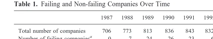
The data for this study consist of 949 listed UK companies in the United Kingdom between 1987–1994. The sample was determined on the basis of availability of data from Datastream. Unfortunately, a complete panel of data was not available for each company in the sample; this means that the total number of companies observed in each year is lower than 949, as shown in the first row of Table 1.4
According to the Stock Exchange Yearbook, there were 160 listed companies that failed between 1987–1994. A company is deemed to have failed if it entered liquidation, receivership or administration as defined by the Yearbook. Financial information for 90 of these companies was found in Datastream. Thus, the frequency of corporate failure in the sample is 1.4% per annum.5
The dependent variable, FAILSit, takes a value of 1 if two requirements are met: first, that the company entered bankruptcy and, secondly, that the company filed its final annual
4Two points should be made about the presence of missing observations in the data. First, the majority of
companies (653) have a complete panel of data covering all eight-years. Secondly, when the sample proportion of companies differs from the population proportion of companies, the logit model has consistent coefficient estimates for all variables except the constant [Anderson (1972)]. The next section shows that the results from the probit and logit models are very similar. Thus, there is strong reason to believe that there are no sample selection problems.
report prior to entering bankruptcy. For companies which did not go bankrupt, and for the earlier reports of failing companies, FAILSit takes a value of 0.
6
The average length of time between the final annual report of a failing company and its entry into bankruptcy was 14 months.7
The number of failures in the population of listed companies, Ft, is included in the bankruptcy model to capture cyclical effects. Rows 2 and 3 of Table 1 highlight the time lag which arose because companies did not immediately enter bankruptcy when they issued their final reports. The data also indicate that companies were more likely to fail in the recession of 1990 –1992 than in the boom of the late 1980s and the economic recovery after 1992. To capture relative changes in business confidence, a variable (CBIt) was constructed from the Confederation of British Industry (CBI) Quarterly Industrial Trends Surveys, in which the CBI published the results of a questionnaire asking the following question: “Are you more, or less, optimistic than you were four months ago about the general business situation in your industry?”8CBItis equal to the proportion of respondents answering “more” minus the proportion answering “less.” Therefore, Ft captures the effect of current economic conditions while CBItis a leading indicator of future changes in economic conditions.
As the probability of bankruptcy is likely to vary across industry sectors, it is important to include industry dummies. The standard industrial classification (SIC) codes were obtained for each company’s main activities from Extel. Data were collected at the one-digit level, with the exception of classification 8500, which refers to companies owning and dealing in real estate. This exception was made because of the volatile nature of the housing market over the period. Table 2 shows the number of companies operating in each industry sector.
Table 3 shows that there are a large number of companies with more than one main activity, reflecting the diversification of many listed companies.
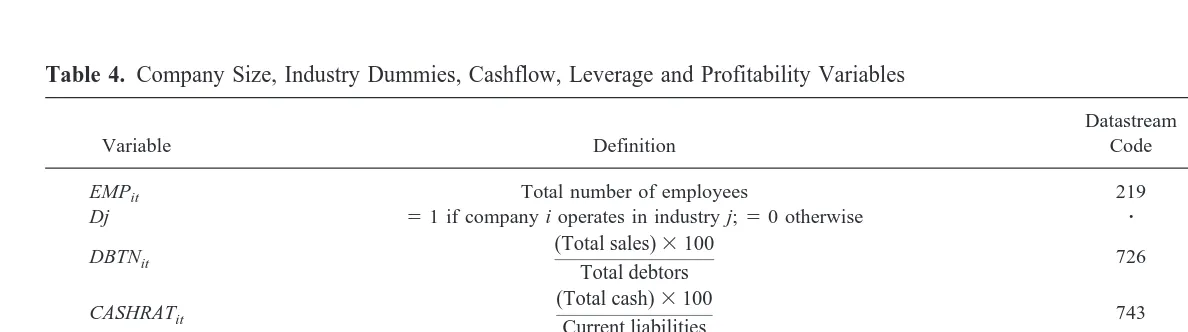
Variables capturing company size, profitability, leverage, and cashflow were collected from Datastream and are defined in Table 4.9The number of employees (EMPit) is used as a measure of company size, and the SIC data are used to create industry dummies (Dj). The debtor-turnover (DBTNit), gross cashflow (GCFit) and cash ratio (CASHRATit)
6None of the failing companies issued reports after filing for bankruptcy. 7This is consistent with the findings of Citron and Taffler (1992). 8For each year, the results from the April questionnaire were used.
9These financial ratios are defined by Datastream to aid analysts in evaluating companies’ financials. They
can be directly downloaded from Datastream without the need for any complex calculations, by using the codes given in Table 4.
Table 1. Failing and Non-failing Companies Over Time
1987 1988 1989 1990 1991 1992 1993 1994 Total
Total number of companies 706 773 813 836 843 832 823 790 6416
Number of failing companiesa 0 7 24 26 23 6 3 1 90
Ft 4 5 6 36 46 41 15 7 160
CBIt 29 18 25 223 217 8 30 13 z
aA company is defined as failing if FAILS it51.
FAILSit51 if company i issued its last annual report in year t, prior to entering bankruptcy;50, otherwise.
Ft5total number of UK listed companies entering bankruptcy in year t.
CBIt5proportion of respondents stating that business conditions had improved over the past four months minus the proportion of respondents stating that business conditions had deteriorated.
variables are used as measures of cashflow. DBTNitcaptures the effect of debtor repay-ment on cashflow; if DBTNit is low, the company may have experienced problems in receiving payment for past sales. GCFit is a measure of profit-generated cashflow. CASHRATitcaptures the ability of the company to meet its short-term liabilities through cash reserves.10
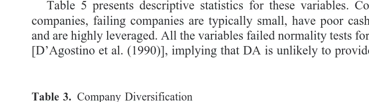
Table 5 presents descriptive statistics for these variables. Compared to non-failing companies, failing companies are typically small, have poor cashflow and profitability, and are highly leveraged. All the variables failed normality tests for skewness and kurtosis [D’Agostino et al. (1990)], implying that DA is unlikely to provide satisfactory results.11
10Previous bankruptcy studies have used very simple ratios; for example, the Zmijewski (1984) model
comprised the return on assets (net income/total assets), the current ratio (current assets/current liabilities) and gearing (debt/total assets). These ratios are not readily available from Datastream and so are not included in the model. Other financial ratios provided by Datastream are income gearing (Datastream code, 732), creditor turnover (728), stock turnover (724), working capital ratio (741), and the quick ratio (742). These variables were found to have insignificant and/or non-constant effects on bankruptcy and were therefore omitted from the model.
11The number of employees (EMP
it), debtor-turnover (DBTNit), and cash ratio (CASHRATit) variables are
inevitably non-normal because they have a lower bound of zero. In addition, the use of industry dummies clearly violates the normality assumption. In this respect, it should be noted that DA may perform quite well when all
Table 3. Company Diversification
Number of Industry Sectors Number of Companies
1 455
2 325
3 146
4 37
5 12
6 1
Total 949
Table 2. Main Activities
SIC Code Industry Sector Number of Companies
0 Agriculture 19
1 Energy and water 31
2 Extraction of minerals and ores 137
3 Metal goods 275
4 Other manufacturing 274
5 Construction 100
6 Distribution, hotels and catering 411
7 Transport and communication 47
8a Banking, finance and insurance 255
8500 Owning and dealing in real estate 151
9 Other services 84
Total 1784b
aClassification 8 refers to all industries with a first digit which begins with an 8, but which does not belong to classification
8500.
bThe total of 1784 is greater than the number of companies in the sample (949) because some companies operated in more
Table 4. Company Size, Industry Dummies, Cashflow, Leverage and Profitability Variables
Variable Definition
Datastream
Code Interpretation
EMPit Total number of employees 219 Company size
Dj 51 if company i operates in industry j;50 otherwise z Industry effects
DBTNit
(Total sales)3100
Total debtors 726 Debtor turnover ratio
CASHRATit
(Total cash)3100
Current liabilities 743 Cash ratio
GCFit
(Profits earned for ordinary shareholders1depreciation1tax equalisation)3100
Capital employed1current liabilities2intangibles 735 Gross cashflow
CAPGit
(Preference capital1subordinated debt1loan capital1short-term borrowings)3100
Capital employed1short-term borrowing2intangibles 731 Capital gearing
ROCit
(Total interest charged1pre-tax profit)3100
Capital employed1short-term borrowing2intangibles 707 Return on capital
Evaluating
Probit,
Logit
and
DA
Approaches
These results were also confirmed using Shapiro and Wilk (1965) and Shapiro and Francia (1972) tests.
IV. Empirical Results
This section presents the results from estimating the following bankruptcy model:
FAILS*it5b1Xit1uit uit,IID~0, exp~2b92Xit!!, (7)
where
FAILSit51 if FAILS*it$0
FAILSit50 otherwise.
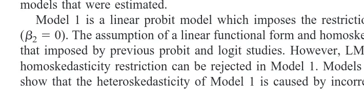
The Xitvariables used to predict bankruptcy are those shown in Tables 1, 2 and 4. Table 6 summarizes the key characteristics and assumptions of the seven probit, logit and DA models that were estimated.
Model 1 is a linear probit model which imposes the restriction of homoskedasticity (b250). The assumption of a linear functional form and homoskedasticity is the same as that imposed by previous probit and logit studies. However, LM tests revealed that the homoskedasticity restriction can be rejected in Model 1. Models 2– 4 were estimated to show that the heteroskedasticity of Model 1 is caused by incorrectly assuming a linear
explanatory variables are dichotomous; however, DA’s performance is less likely to be satisfactory when variables have a lower bound [Amemiya and Powell (1983)].
Table 6. Summary of Models 1–7
Model
Assumes Normality and Equal Group Covariance Matrices?
Functional Form
Assumes Homoskedasticity?
Distribution of uit
1. Linear homoskedastic probit No Linear Yes Normal
2. Linear heteroskedastic probit No Linear No Normal
3. Non-linear heteroskedastic probit No Non-linear No Normal
4. Non-linear homoskedastic probit No Non-linear Yes Normal
5. Non-linear homoskedastic logit No Non-linear Yes Logistic
6. Discriminant analysis Yes Non-linear No Not applicable
Table 5. Descriptive Statistics
Variables
Non-Failing Companies (Number of Observations56326)
Failing Companies (Number of Observations590)
Mean Standard Deviation Mean Standard Deviation
EMPit 6399.26 20160.45 1176.50 2244.24
DBTNit 827.59 1646.87 580.52 532.46
CASHRATit 33.98 90.50 10.46 18.31
GCFit 9.22 10.03 20.87 14.78
CAPGit 3062.15 8699.26 11008.68 28528.21
functional form. In particular, the gross cashflow (GCFit) and leverage (CAPGit) variables have non-linear effects. Model 3 is the most general model, as it allows for non-linearities and heteroskedasticity. Once the non-linear effects of GCFit and CAPGit are taken into account, the null hypothesis of homoskedasticity can no longer be rejected. Therefore, the homoskedasticity restriction can be imposed, as in Models 4 and 5. Models 4 and 5 enable a comparison of the logit and probit results to investigate whether the choice between the logistic and normal distributions is important.
Table 7 presents the results for the probit and logit models. The LM1 test statistics indicate no problems of omitted variable bias; however, Model 1’s LM2 statistic shows that the null hypothesis of homoskedasticity is rejected in the linear model. The signifi-cance of the gross cashflow (GCFit) and leverage (CAPGit) variables in the heteroske-dastic part of Model 2 confirms that these variables were the cause of the heteroskedas-ticity in Model 1.
The LM test for heteroskedasticity indicates that a non-constant variance for the residuals can be caused by imposing an incorrect functional form.12 To investigate whether leverage and cashflow have non-linear effects, polynomial terms in CAPGitand GCFitwere added in Model 3. Model 3 is the least restrictive, because it allows for both polynomial terms in CAPGit and GCFit and for heteroskedasticity. These polynomial terms have highly significant effects, and including them means that one can no longer reject the null hypothesis of homoskedasticity (b250). The LM2 test statistics for Models 4 and 5 confirm that once the non-linear effects of cashflow and leverage are taken into account, the null hypothesis of homoskedasticity can no longer be rejected. The results for Models 4 and 5 are very similar, indicating that there is little to choose between the probit and logit approaches.
The results show that bankruptcy is more likely when the economy moves from boom to recession. The negative coefficient on the number of failing companies in the popula-tion (Ft) implies that a company is less likely to go bankrupt in the future if the economy is currently in a recession. The negative coefficient on the CBI indicator (CBIt) implies that an improvement in business confidence is correlated with a fall in the probability of bankruptcy (an increase in CBItimplies that business confidence is improving). The signs on Ft and CBIt show that a company is less (more) likely to fail over the next 12–18 months if the economy is currently in a recession (boom) and business conditions are expected to improve (worsen).
Another important determinant of bankruptcy is company size. The coefficient on the number of employees (EMPit) is negative, showing that corporate failure is more likely if a company is small.13 The industry dummies are also important; a company was more likely to enter bankruptcy if it operated in the construction (D5i) or financial services (D8i) sectors. This reflects the fact that high interest rates badly affected the building industry and, in contrast to the 1979 –1981 recession, the 1990 –1992 recession badly hit the financial services sector.
12Equation (6) shows that the heteroskedasticity may be captured by including polynomial terms rather than
by allowing the error term to have a non-constant variance.
13It might be argued that company size can affect the probability of bankruptcy because large companies
tend to be more highly diversified and are less vulnerable to sector-specific shocks. To investigate this possibility, a variable capturing the number of industry sectors in which companies had main activities was included in the model. No evidence was found to suggest that the degree of diversification helped improve predictive accuracy.
Table 7. Probit and Logit Models of Bankruptcy 1987–1994 ( z statistics in parentheses)
FAILS*it5b91Xit1uit uit,IID~0, exp~2b92Xit!!
Explanatory Variables Model 1 Model 2 Model 3 Model 4 Model 5
Ft 20.011 20.019 20.016 20.015 20.034
(22.880) (23.585) (23.397) (23.682) (23.506)
CBIt 20.026 20.036 20.030 20.030 20.065
(26.697) (25.912) (25.287) (26.775) (26.494)
EMPit 20.379e-04 20.582e-04 20.457e-04 20.455e-04 21.013e-04
(22.193) (22.204) (22.201) (22.342) (22.175)
D1i 0.451 0.617 0.545 0.540 1.199
(1.744) (1.974) (1.990) (2.127) (2.111)
D2i 20.239 20.183 20.144 20.145 20.376
(21.420) (20.860) (20.807) (20.812) (20.886)
D4i 0.084 0.138 0.108 0.108 0.299
(0.746) (0.922) (0.856) (0.865) (1.803)
D5i 0.416 0.530 0.457 0.455 0.959
(3.116) (2.930) (2.888) (3.103) (3.077)
D8i 0.399 0.462 0.394 0.392 0.840
(3.800) (3.183) (3.064) (3.339) (3.282)
D8500i 20.054 20.119 20.186 20.185 20.362
(20.408) (20.660) (21.239) (21.260) (21.104)
DBTNit 20.205e-03 20.255e-03 20.227e-03 20.226e-03 20.499e-03
(21.876) (21.606) (21.789) (21.804) (21.718)
CASHRATit 20.777e-02 20.4592 20.355e-02 20.353e-02 20.955e-02
(23.296) (21.808) (21.602) (21.627) (21.769)
GCFit 20.177e-01 0.761e-02 20.122e-01 20.117e-01 20.281e-01
(25.272) (0.643) (20.896) (21.250) (21.413)
GCFit
2
z z 20.283e-03 20.279e-03 20.657e-03
z z (21.838) (22.020) (22.089)
CAPGit 0.116e-04 0.513e-04 0.254e-03 0.254e-03 0.539e-03
(3.842) (2.054) (6.789) (6.986) (6.807)
CAPGit
2
z z 20.848e-08 20.849e-08 21.800e-08
z z (24.622) (24.662) (24.650)
z z 20.115e-18 20.116e-18 20.245e-18
z z (22.365) (23.171) (23.218)
ROCit 0.960e-06 20.632e-04 20.639e-04 20.638e-04 21.218e-04
(0.154) (22.307) (21.776) (21.821) (21.767)
Constant 21.759 22.267 22.533 22.529 24.952
(212.591) (29.247) (210.584) (211.324) (29.789) Heteroskedasticity
GCFit z 20.992e-02 0.300e-03 z z
z (22.793) (0.050) z z
CAPGit z 0.501e-04 0.571e-06 z z
z (3.823) (0.032) z z
LM1a 1.050
z z 0.025 1.145
95% critical value 6.571 z z 9.390 9.390
LM2b 49.979
z z 9.663 14.168
95% critical value 16.928 z z 23.300 23.300
Pseudo R2 0.2169
z z 0.3305 0.3249
aLM1: LM test for omitted variable bias.
bLM2: LM test for heteroskedasticity and incorrect functional form.
A company is also more likely to go bankrupt when it is suffering cashflow difficulties. The negative coefficient on the debtor-turnover ratio (DBTNit) implies that a company is more likely to fail if it is having problems receiving payment from debtors. Similarly, the negative coefficient on the cash ratio (CASHRATit) indicates that companies are more likely to fail if cash reserves are low. The negative coefficient on gross cashflow (GCFit) shows that a company is more likely to go bankrupt when profit-generated cashflow is low.
Models 3–5 show that GCFithas non-linear effects on FAILS*it. Differentiating FAILS*it with respect to GCFitshows how a change in gross cashflow affects the probability of bankruptcy. For values of GCFitthat lie within two standard deviations of the mean of GCFit, an increase in cashflow always reduces the probability of bankruptcy. However, the size of this effect depends on whether the company is suffering from cashflow problems. For low values of GCFit, an increase in cashflow has a small negative effect on the probability of bankruptcy; for high values of GCFit, an increase in cashflow has a large negative effect. In other words, companies are less likely to go bankrupt as cashflow improves, and this effect is larger for companies with relatively healthy cashflow.
Company indebtedness is also an important determinant of bankruptcy. The positive coefficient on capital gearing (CAPGit) in Model 1 shows that a company is more likely to fail when leverage is high. Models 3– 6 show that there is a non-linear relationship between leverage and bankruptcy. Differentiating FAILS*itwith respect to CAPGitshows how a change in leverage affects the probability of bankruptcy. For values of CAPGitthat lie within two standard deviations of the mean of CAPGit, an increase in leverage always increases the probability of bankruptcy. For low values of CAPGit, an increase in leverage has a large positive effect on the probability of bankruptcy. For high values of CAPGit, an increase in leverage has a small positive effect on the probability of bankruptcy. Thus, an increase in leverage raises the probability of bankruptcy, but this effect diminishes as leverage increases.14
The negative coefficient on the return on capital (ROCit) means that a company is more likely to fail when profitability is low. It is noteworthy that the profitability effect is absent in Model 1, which incorrectly assumes a linear functional form, and is only detected when the non-linear effects of leverage and cashflow are taken into account. This emphasizes the importance of testing for heteroskedasticity.
To summarize, a company is most likely to go bankrupt when it is unprofitable, highly leveraged, and has cashflow problems.15 Although these results are similar to those of previous studies, the finding of non-linear effects for cashflow and leverage is new. These non-linear effects were only discovered by testing for heteroskedasticity. This reinforces the importance of testing for misspecification in probit and logit models. In contrast to studies using the matching approach, company size, industry sector and the economic cycle have also been shown to have important effects on the probability of bankruptcy.
14A relatively small proportion of the observations for GCF
it(6.9%) and CAPGit(0.3%) took negative
values. For these observations, the interpretation of the coefficients on the second and fourth powers is less clear than for positive observations. Various checks were carried out to ensure that this was not a major problem. Omitting the small number of negative CAPGitobservations had no effect on the sign or significance of the
coefficients on CAPGit
2or CAPG
it
4. Similarly, omitting the negative GCF
itobservations had no effect on the sign
or significance of GCFit2(however, omitting negative GCFitobservations involved dropping 34 failing
obser-vations and resulted in a less robust model). Retaining negative obserobser-vations but omitting the CAPGit
2, CAPG
it
4
and GCFit2variables was not found to solve the heteroskedasticity problem, and so it seemed sensible to retain
these polynomial terms.
15It should be noted that lagged variables were not found to be important predictors of bankruptcy.
Having developed a model of bankruptcy which appears to be well-specified, the analysis turns to consider the results from DA, so as to evaluate whether there are gains in predictive accuracy from using probit and logit rather than DA. Table 8 reports the results using DA (Model 6), where cashflow and leverage are allowed to have non-linear effects as in Models 4 and 5.16 Panel A shows that the eigenvalue and canonical correlation statistics are rather low, suggesting that the DA model is not exceptionally good at discriminating between the samples of failing and non-failing companies. The significance of the Wilks’ lambda statistic shows that the null hypothesis that the mean of the discriminant scores is the same in the groups of failing and non-failing companies can
16The estimation results for the DA model are shown separately from those for the probit and logit models,
as the reported test statistics are somewhat different.
Table 8. Results for DA (Model 6)a
Panel A: Canonical Discriminant Functions
Eigenvalueb Canonical Correlationc Wilks’ Lambdad x2(18) Prob.x2
0.048 0.214 0.954 300.555 0.000
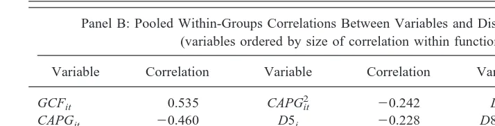
Panel B: Pooled Within-Groups Correlations Between Variables and Discriminant Function (variables ordered by size of correlation within function)
Variable Correlation Variable Correlation Variable Correlation
GCFit 0.535 CAPGit2 20.242 D2i 0.117
CAPGit 20.460 D5i 20.228 D8500i 20.089
CBIt 0.445 Ft 20.221 DBTNit 0.081
CAPGit3 20.272 CASHRATit 0.141 D1i 20.049
CAPGit4 20.270 EMPit 0.140 D4i 0.035
D8i 20.265 ROCit 0.127 GCFit2 20.022
Panel C: Test of Equality of Group Covariance Matrices Using Box’s M
(the ranks and natural logarithms of determinants are those of the group covariance matrices)
Group Rank Log Determinant
FAILSit50 18 291.02
FAILSit51 18 260.04
Pooled within-groups
covariance matrix 18 293.06
Box’s M Approximate F(171) Significance Prob.F Number of Observations
15480 86.013 72733.4 0.000 6416
aDA calculatesb
i(i51, . . . , n), giving a Z score which can be used to classify observations into one of the two samples:
Z5b1X11b2X21. . .1bnXn.
These weights were estimated so that they resulted in the best separation between the samples, given prior probabilities and costs of misclassification. In other words, the weights were chosen so as to maximize the (between-groups sum of squares/ within-groups sum of squares) ratio.
bEigenvalue[(between group sum of squares/within group sum of squares). cCanonical correlation[(between group sum of squares/total sum of squares)1/2.
In the two group case, the canonical correlation is the correlation coefficient between the discriminant score and the group variable.
dWilks’ lambda[(within group sum of squares/total sum of squares).
be rejected. Panel B assesses the contribution of each variable to the discriminant function. Selecting variables on the basis of each variable’s contribution to the discriminant function resulted in models with low explanatory power. Moreover, the size of the correlation between each variable and the discriminant function did not reflect the levels of significance in the probit model and logit models. This suggests that the level of correlation with the discriminant function is a poor criterion for choosing which variables should be included in the model.
Box’s M tests the null hypothesis of equal covariance matrices assuming multivariate normality. Panel C shows that the null hypothesis of equality in the group covariance matrices can be strongly rejected. This may be due either to a failure of multivariate normality or because the group covariance matrices are not equal. In either case, the DA approach, together with a linear classification rule, is not an appropriate way in which to estimate the bankruptcy model.
V. Explanatory Power
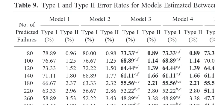
In evaluating the explanatory power of the bankruptcy models, it is helpful to define two types of prediction error. A type I error occurs when a company fails but is predicted to survive; a type II error occurs when a company survives but is predicted to fail. Clearly, the type I and type II error rates depend on the number of companies predicted to fail. The higher (lower) the number of companies predicted to go bankrupt, the smaller (larger) is the type I error rate and the larger (smaller) is the type II error rate. The number of predicted bankruptcies depends on the cut-off probabilities chosen for the models. For example, if the cut-off is equal to 0.1, a company for which the expected probability of bankruptcy exceeds 10% is predicted to go bankrupt, whereas a company for which the expected probability of bankruptcy is less than 10% is predicted to survive. One can therefore increase the number of companies predicted to fail by reducing the cut-off probability. Table 9 presents the type I and type II error rates for the probit, logit and DA models for different cut-offs; the lowest type I and type II error rates are highlighted in bold.
In comparing these results to previous studies, it is important to note that reported type I and type II error rates depend critically on the sample selection criterion. Studies which sample approximately equal numbers of failing and non-failing companies typically have much smaller error rates compared to those where the sample frequency of failure is close to the population frequency, as in this study [see Zmijewski (1984, Table 1)]. The type I and II error rates reported in this paper are comparable to those of previous studies with sample frequency failure rates of less than 3% [White and Turnbull (1975); Zmijewski (1983)].
The results indicate that the non-linear models (3, 4 and 5) predicted better than the linear models (1 and 2). This shows that a failure to take account of the non-linear effects of cashflow and leverage results in models with worse explanatory power. Models 3–5 also had lower type I and type II error rates than Model 6, suggesting that well-specified probit and logit models are superior to the DA model. For all cut-off probabilities, the type I error rates of Models 3–5 were significantly less than those of Models 1 and 6 (at confidence levels of at least 80%); the differences between the type II error rates were not statistically significant. As type I errors tend to be much more costly than type II errors,
this suggests that there may be real gains to users when models are tested for misspeci-fication problems.17
It is worth noting that the type I and type II error rates of Models 1 and 2 are very similar to those of Model 6. In other words, there is virtually no difference between the explanatory power of misspecified probit models and the DA model. This reflects the findings of previous studies which argued that there is little gain from using probit or logit approaches rather than DA [Press and Wilson (1978); Lo (1986); Collins and Green (1982)]; however, these studies did not test the probit and logit models for omitted variable bias or heteroskedasticity and did not allow for non-linear effects.
Table 10 shows how Model 5’s accuracy was affected by alternative bankruptcy horizons. The benchmark case is where the model predicts one period ahead (the error rates for column 1 correspond to those reported in Table 9). The second (third and fourth) column(s) show Model 5’s type I and type II error rates for failures predicted to occur within the next two (three and four) reporting periods.
Consistent with previous research, the bankruptcy model showed a decline in accuracy for more distant bankruptcy horizons. However, the deterioration in accuracy was not very great; for example, a comparison of Tables 9 and 10 shows that Model 5 had lower type I and type II error rates, when the bankruptcy horizon was two periods, than DA where the horizon was just one period.
17Altman (1977) estimated the relative costs of type I and type II errors for commercial bank loans as being
7:1.
Table 9. Type I and Type II Error Rates for Models Estimated Between 1987–1994
No. of Predicted
Failures
Model 1 Model 2 Model 3 Model 4 Model 5 Model 6
Type I
80 78.89 0.96 80.00 0.98 73.33c,f 0.89 73.33c,f 0.89 73.33c,f 0.89 78.89 0.96
100 76.67 1.25 76.67 1.25 68.89c,f 1.14 68.89c,f 1.14 70.00c,f 1.15 76.67 1.25
120 73.33 1.52 72.22 1.50 64.44c,f 1.39 64.44c,f 1.39 64.44c,f 1.39 72.22 1.50
140 71.11 1.80 68.89 1.77 61.11c,f 1.66 61.11c,f 1.66 61.11c,f 1.66 70.00 1.79
180 66.67 2.37 63.33 2.32 55.56b,e 2.21 55.56b,e 2.21 55.56b,e 2.21 65.56 2.36
220 63.33 2.96 56.67 2.86 52.22b,e 2.80 52.22b,e 2.80 51.11a,d 2.78 63.33 2.96
260 58.89 3.53 52.22 3.43 48.89c,f 3.38 48.89c,f 3.38 47.78c,f 3.37 56.67 3.49
300 54.44 4.09 51.11 4.05 42.22b,e 3.92 42.22b,e 3.92 41.11b,e 3.90 52.22 4.06
500 43.33 7.10 36.67 7.00 32.22b,e 6.94 31.11b,e 6.92 32.22b,e 6.94 42.22 7.08
1000 30.00 14.81 14.44 14.59 13.33a,d 14.57 13.33a,d 14.57 13.33a,d 14.57 25.56 14.75
2000 13.33 30.38 7.78 30.30 6.67b,e 30.29 6.67b,e 30.29 6.67b,e 30.29 13.33 30.38
4000 1.11 61.82 0c,f 61.81 0c,f 61.81 0c,f 61.81 0c,f 61.81 1.11 61.82
Total number of observations56416. Number of failures590.
aSignificantly lower than corresponding error rate for Model 6 at 95% confidence level (one-tailed test).
bSignificantly lower than corresponding error rate for Model 6 at 90% confidence level (one-tailed test).
cSignificantly lower than corresponding error rate for Model 6 at 80% confidence level (one-tailed test).
dSignificantly lower than corresponding error rate for Model 1 at 95% confidence level (one-tailed test).
eSignificantly lower than corresponding error rate for Model 1 at 90% confidence level (one-tailed test).
To evaluate out-of-sample accuracy, Models 1– 6 were re-estimated using data for 1987–1990, and were used to identify failing companies between 1991–1994.18Table 11 shows the type I and type II error rates for these re-estimated models during the hold-out period (1991–1994). A comparison of Tables 9 and 11 show that there is little difference between the accuracy of models in the estimation and hold-out samples. This suggests that the models do not suffer from over-fitting.
As in Table 9, the non-linear models (3, 4 and 5) generally performed better than the DA model (Model 6). The difference in type I error rates was statistically significant (at the 95% confidence level) for the 20 – 40 observations with the highest predicted bank-ruptcy probabilities. This suggests that the difference in accuracy is greatest when the number of predicted failures is close to the number of actual failures (33 in the hold-out sample). The difference in accuracy between the linear and non-linear probit models was not statistically significant in the hold-out sample. The linear models (1 and 2) generally performed better than DA, but their superior performance was less significant statistically. This is consistent with previous studies which imposed linear specifications and did not find significant differences between the probit, logit and DA approaches.
18The Lachenbruch approach does not accurately measure explanatory power when coefficients are
non-constant over the sample period. Therefore, a hold-out sample was used in preference to the Lachenbruch method.
Table 10. Type I and Type II Error Rates of Model 5 for Alternative Bankruptcy Horizons
No. of Predicted
Failures
Number of Reporting Periods Prior to Failure
One Perioda Two Periodsb Three Periodsc Four Periodsd
Type I
80 73.33 0.89 79.21 0.69 83.53 0.62 86.23 0.62
100 70.00 1.15 78.84 0.91 81.18 0.84 84.26 0.81
120 64.44 1.39 73.03 1.15 78.82 1.07 82.30 1.08
140 61.11 1.66 70.79 1.41 76.86 1.31 80.66 1.33
180 55.56 2.21 65.73 1.91 71.76 1.75 76.07 1.75
220 51.11 2.78 62.36 2.45 69.02 2.29 73.11 2.26
260 47.78 3.37 58.43 2.98 66.27 2.82 70.49 2.78
300 41.11 3.90 52.81 3.46 61.96 3.29 66.56 3.24
500 32.22 6.94 41.57 6.35 51.37 6.10 57.05 6.04
1000 13.33 14.57 25.28 13.90 36.08 13.59 42.30 13.48
2000 6.67 30.29 16.29 29.67 24.31 29.33 30.49 29.26
4000 0 61.81 4.49 61.40 7.45 61.09 9.84 60.96
aThere were 90 observations where companies issued their final reports prior to entering bankruptcy (i.e., where FAILS it5 1).
bThere were 178 observations where companies issued their final or penultimate reports prior to entering bankruptcy (i.e.,
where FAILSit215FAILSit51).
cThere were 255 observations where companies issued their last three reports prior to entering bankruptcy (i.e., where
FAILSit225FAILSit215FAILSit51).
dThere were 305 observations where companies issued their last four reports prior to entering bankruptcy (i.e., where
FAILSit235FAILSit225FAILSit215FAILSit51).
For each cut-off, the type I error rate tended to rise and the type II error rate fell as the bankruptcy horizon increased. This means that a statistical test for each cut-off, similar to those reported in Tables 9 and 11, would not be meaningful. This is because, as the bankruptcy horizon increased, the number of failing observations rose (from 90 to 305), whereas the number of predicted failures was constant for each cut-off.
VI. Conclusion
Consistent with previous research, this study has shown that profitability, leverage and cashflow have important effects on the probability of bankruptcy. Whereas previous studies did not report tests for misspecification, heteroskedasticity tests used in this paper revealed that cashflow and leverage have non-linear effects on the probability of bank-ruptcy; incorporating these effects into the model improved its predictive accuracy. In contrast to previous studies, this paper avoided the matching approach. Therefore, it was able to evaluate the effects of company size, industry sector, and the economic cycle on the probability of bankruptcy, and avoided the over-fitting problems which can arise in small samples.
In contrast to previous studies, probit and logit models were found to perform better than DA. In hold-out samples, this difference in predictive accuracy was found to be greatest for realistic cut-off probabilities (where the numbers of predicted and actual failures were similar), and for type I errors (which, in practice, are much more costly than type II errors). Moreover, this superiority over DA was greatest for well-specified non-linear probit and logit models. This may explain why previous studies which did not report tests for misspecification found that probit, logit and DA models were very similar in terms of predictive accuracy.
References
Aghion, P., and Bolton, P. July 1992. An “incomplete contracts” approach to financial contracting. Review of Economic Studies 59(3):473–494.
Table 11. Type I and Type II Error Rates in Hold-out Sample (1991–1994) for Models
Estimated Between 1987–1990
No. of Predicted
Failures
Model 1 Model 2 Model 3 Model 4 Model 5 Model 6
Type I
60 63.64 1.47 63.64 1.47 69.70 1.54 63.64 1.47 66.67 1.51 72.73 1.57 80 57.58 2.03 60.61 2.06 63.64 2.09 63.64 2.09 63.64 2.09 66.67 2.12 100 54.54 2.61 51.52 2.58 57.58 2.64 57.58 2.64 60.61 2.67 60.61 2.67 120 54.54 3.23 48.48 3.16 51.52 3.20 51.52 3.20 51.52 3.20 57.58 3.26 140 45.45 3.75 48.48 3.78 45.45 3.75 42.42 3.72 45.45 3.75 57.58 3.87 160 42.42 4.33 48.48 4.39 39.39 4.30 36.36 4.27 39.39 4.30 51.52 4.42 180 42.42 4.95 48.48 5.01 36.36 4.88 36.36 4.88 33.33 4.85 42.42 4.95 200 42.42 5.56 48.48 5.62 36.36 5.50 36.36 5.50 33.33 5.47 36.36 5.50 240 36.36 6.73 39.39 6.76 33.33 6.70 33.33 6.70 30.30 6.67 33.33 6.70 300 33.33 8.54 36.36 8.57 27.27 8.48 27.27 8.48 30.30 8.51 30.30 8.51 500 24.24 14.59 27.27 14.62 24.24 14.59 24.24 14.59 24.24 14.59 21.21 14.56 1000 18.18 29.89 15.15 29.86 12.12 29.83 12.12 29.83 12.12 29.83 12.12 29.83
Number of observations in hold-out sample53288. Number of failures in hold-out sample533. aSignificantly lower than corresponding error rate for Model 6 at 95% confidence level (one-tailed test).
bSignificantly lower than corresponding error rate for Model 6 at 90% confidence level (one-tailed test).
Altman, E. I. Sept. 1968. Financial ratios, discriminant analysis and the prediction of corporate bankruptcy. Journal of Finance 23: 589–609.
Altman, E. I., Haldeman, R. G., and Narayanan, P. June 1977. Zeta analysis. Journal of Banking and Finance: 29–54.
Altman, E. October 1977. Some estimates of the cost of lending errors for commercial banks. Journal of Commercial Bank Lending: 51–58.
Altman, E. 1986. Financial ratios, discriminant analysis and the prediction of corporate bankruptcy. In Issues and Readings in Managerial Finance (R. E. Johnson, ed.). New York: Dryden Press, pp. 53–75
Amemiya, T., and Powell, J. 1983. A comparison of the logit model and normal discriminant analysis when the independent variables are binary. In Studies in Econometrics, Time Series, and Multivariate Statistics (S. Karlin, T. Amemiya and L. A. Goodman, eds.). New York: Academic Press, pp. 1–24
Anderson, J. A. 1972. Separate sample logistic discrimination. Biometrika 59(1):19–35.
Beaver, W. H. 1966. Financial ratios as predictors of bankruptcy. Journal of Accounting Research (Supplement):71–102.
Blum, M. Spring 1974. Failing company discriminant analysis. Journal of Accounting Research 12(1):1–25.
Bulow, J., and Shoven, J. Autumn 1978. The bankruptcy decision. The Bell Journal of Economics 9(2):437–456.
Citron, D., and Taffler, R. J. Autumn 1992. The audit report under going concern uncertainties: An empirical analysis. Accounting and Business Research 22:337–345.
Collins, R., and Green, R. 1982. Statistical methods for bankruptcy prediction. Journal of Econom-ics and Business 34(4):349–354.
D’Agostino, R. B., Balanger, A., and D’Agostino, Jr., R. B. Nov. 1990. A suggestion for using powerful and informative tests of normality. The American Statistician 44:316–321.
Davidson, R., and MacKinnon, J. G. July 1984. Convenient specification tests for logit and probit models. Journal of Econometrics 25(3):241–262.
Deakin, E. B. Spring 1972. A discriminant analysis of predictors of business failure. Journal of Accounting Research 10:167–179.
Dixit, A., and Pindyck, R. 1994. Investment Under Uncertainty. Princeton: Princeton University Press.
Eisenbeis, R. A. June 1977. Pitfalls in the application of discriminant analysis in business, finance and economics. Journal of Finance 22(3):875–890.
Elam, R. Jan. 1975. The effect of lease data on the predictive ability of financial ratios. The Accounting Review 5(1): 25–43.
Hamer, M. 1983. Failure prediction: Sensitivity of classification accuracy to alternative statistical methods and variable sets. Journal of Accounting and Public Policy 2:289–307.
Hart, O. 1995. Firms, Contracts and Financial Structure. Oxford: Clarendon Lectures in Econom-ics, OUP.
Hopwood, W. S., McKeown, J. C., and Mutchler, J. F. 1994. A Re-examination of auditor versus model accuracy within the context of the going-concern opinion decision. Contemporary Accounting Research 10(2):409–431.
Hubbard, G. December 1994. Investment under uncertainty: Keeping one’s options open. Journal of Economic Literature 32(4):1816–1831.
Jones, F. L. 1987. Current techniques in bankruptcy prediction. Journal of Accounting Literature 6:131–164.
Koh, H. C. Autumn 1991. Model predictions and auditor assessments of going concern status. Accounting and Business Research 21(84):331–338.
Lachenbruch, P. A. 1975. Discriminant Analysis. Hafner Press. New York
Lo, A. W. March 1986. Logit versus discriminant analysis: A specification test and application to corporate bankruptcies. Journal of Econometrics 31(2):151–178.
McLeay, S. Summer 1986. Student’s t and the distribution of financial ratios. Journal of Business Finance and Accounting 13(2): 209–222.
Morris, R. 1997. Early Warning Indicators of Corporate Failure: A Critical Review of Previous Research and Further Empirical Evidence. Ashgate Publishing in association with the Institute of Chartered Accountants in England and Wales. Aldershot, England.
Myers, S. November 1977. Determinants of corporate borrowing. Journal of Financial Economics 5(2):147–175.
Norton, C. L., and Smith, R. E. Jan. 1979. A comparison of general price level and historical cost financial statements in the prediction of bankruptcy. The Accounting Review 54:72–87. Ohlson, J. S. 1980. Financial ratios and the probabilistic prediction of bankruptcy. Journal of
Accounting Research 18(1):109–131.
Platt, H., Platt, M., and Pedersen, J. June 1994. Bankruptcy discrimination with real variables. Journal of Business, Finance and Accounting 21(4):491–510.
Press, J., and Wilson, S. Dec. 1978. Choosing between logistic regression and discriminant analysis. Journal of the American Statistical Association 73(364): 699–705.
Shapiro, S. S., and Francia, R. S. 1972. An approximate analysis of variance test for normality. Journal of the American Statistical Association 67(337):215–216.
Shapiro, S. S., and Wilk, M. B. 1965. An analysis of variance test for normality. Biometrika 52(3):591–611.
White, R. W., and Turnbull, H. 1975. The probability of bankruptcy for American Industrial Firms. Working paper. London Graduate School of Business.
Wilcox, J. W. 1973. A prediction of business failure using accounting data. Journal of Accounting Research (Supplement) 11:163–179.
Yatchew, A., and Griliches, Z. February 1985. Specification error in probit models. The Review of Economics and Statistics 66(1):134–139.
Zmijewski, M. E. 1983. Essays on corporate bankruptcy. Ph.D. dissertation. State University of New York at Buffalo.