Fundamentals of Digital Image Processing

Fundamentals

of Digital

Image Processing

ANIL K. JAIN

University of California, Davis

8.1 INTRODUCTION

8

I mage Filtering

and

Restoration

Any image acquired by optical, electro-optical or electronic means is likely to be degraded by the sensing environment. The degradations may pe in the form of sensor noise, blur due to camera misfocus, relative object-camera motion, random atmospheric turbulence, and so on. Image restoration is concerned with filtering the observed image to minimize the effect of degradations (Fig. 8.1). _{The effectiveness} of image restoration filters depends on the extent and the accuracy of the knowl­ edge of the degradation process as well as on the filter design criterion. A frequently used criterion is the mean square error. Although, as a global measure of visual fidelity, its validity is questionable (see Chapter 3) _{it is a reasonable local measure} and is mathematically tractable. Other criteria such as weighted mean square and maximum entropy are also used, although less frequently.

Image restoration differs from image enhancement in that the latter is concerned more with accentuation or extraction of image features rather than restoration of degradations. Image restoration problems can be quantified pre­ cisely, whereas enhancement criteria are difficult to represent mathematically. Consequently, restoration techniques often depend only on the class or ensemble

u(x, _{y) I maging}

system

A to D conversion

v(m, n) _Digital

fi lter

u(m, n) _{D to A}

conversion

Display or record

Figure 8.1 Digital image restoration system.

Image restoration

Restoration models Linear filtering Other methods

• Image formation models • l nverse/pseudoinverse filter

• Wiener filter

• Generalized Wiener filter

• Maximum entropy restoration • Bayesian methods

• Spline interpolation/smoothing

• Least squares and SVD, methods

• Coordinate transformation and geometric correction

• Recursive ( Kalman) filter • Semirecursive filter

Figure 8.2 Image restoration.

• Blind deconvolution • Extrapolation and

super-resolution

properties of a data set, whereas image enhancement techniques are much more image dependent. Figure 8-2 summarizes several restoration techniques that are discussed in this chapter.

8.2 IMAGE OBSERVATION MODELS

A typical imaging system consists of an image formation system, a detector, and a recorder. For example, an electro-optical system such as the television camera contains an optical system that focuses an image on a photoelectric device, which is scanned for transmission or recording of the image. Similarly, an ordinary camera uses a lens to form an image that is detected and recorded on a photosensitive film. A general model for such systems (Fig. 8.3) can be expressed as Figure 8.3 Image observation model.

where

u(x,y)

represents the object (also called the original image), and v(x

,

y

) is the observed image. The image formation process can often be modeled by the linear system of

(8.2),

where

h (x, y; x ', y ')

is its impulse response. For space invari­ ant systems, we can write

h(x,y;x',y') =h(x -x',y -y';O,O) �h(x -x',y -y') (8.4)

The functions f ( ·) and g ( ·) are generally nonlinear and represent the characteristics of the detector/recording mechanisms. The term

11(x, y)

represents the additive noise, which has an image-dependent random component f[ g (w)]111 and an image­ independent random component 112•

Image Formation Models

Table

8.1

lists impulse response models for several spatially invariant systems. Diffraction-limited coherent systems have the effect of being ideal low-pass filters. For an incoherent system, this means band-limitedness and a frequency response obtained by convolving the coherent transfer function (CTF) with itself (Fig.

8.4).

Degradations due to phase distortion in the CTF are called aberrations and manifest themselves as distortions in the pass-band of the incoherent optical transfer function (OTF). For example, a severely out-of-focus lens with rectangular aperture causes an aberration in the OTF, as shown in Fig.

8.4.

Motion blur occurs when there is relative motion between the object and the camera during exposure. Atmospheric turbulence is due to random variations in the refractive index of the medium between the object and the imaging system. Such degradations occur in the imaging of astronomical objects. Image blurring also occurs in image acquisition by scanners in which the image pixels are integrated over the scanning aperture. Examples of this can be found in image acquisition by radar, beam-forming arrays, and conventional image display systems using

tele-TABLE 8.1 Examples of Spatially I nvariant Models

Type of system

Sec. 8.2 Image Observation Models

H(�1 • 0)

- 1 .0 -0.5

CTF of a coherent diffraction limited system OTF of an incoherent diffraction limited system Aberration due to severely out-of-focus lens

0.5

1.0

�1

Figure 8.4 Degradations due to diffraction limitedness and lens aberration.

vision rasters. In the case of CCD arrays used for image acquisition, local inter­ actions between adjacent array elements blur the image.

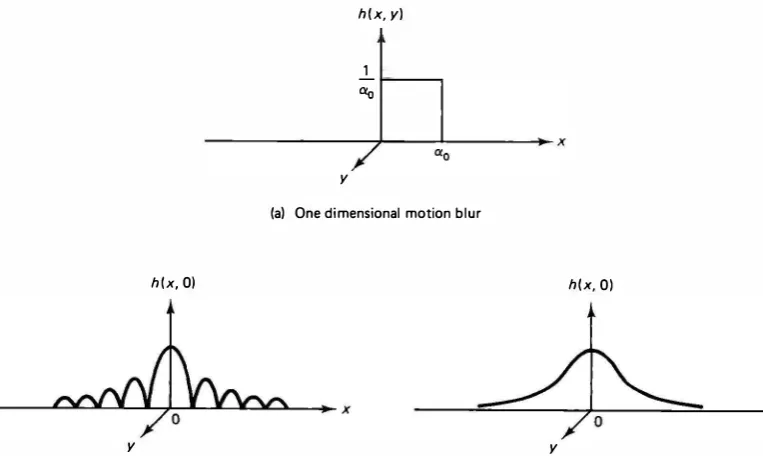
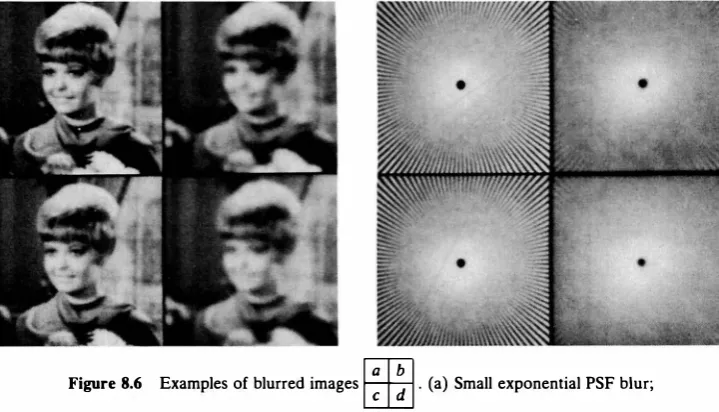
Figure 8.5 shows the PSFs of some of these degradation phenomena. For an ideal imaging system, the impulse response is the infinitesimally thin Dirac delta function having an infinite passband. Hence, the extent of blur introduced by a system can be judged by the shape and width of the PSF. Alternatively, the pass­ band of the frequency response can be used to judge the extent of blur or the resolution of the system. Figures 2.2 and 2.5 show the PSFs and MTFs due to atmospheric turbulence and diffraction-limited systems. Figure 8.6 shows examples of blurred images.

h (x, 0)

y

y h ( x, y)

1 %

(a) One dimensional motion blur

h(x, 0)

y

(bl Incoherent diffraction limited system ( lens cutoff) (c) Average atmospheric turbulence

Figure 8.5 Examples of spatially invariant PSFs.

Figure 8.6 Examples of blurred images

�

. (a) Small exponential PSF blur;

(b) large exponential PSF blur; (c) small sinc2 PSF blur; (d) large sinc2 PSF blur.

Example 8.1

An object u (x, y) being imaged moves uniformly in the x-direction at a velocity " . If the exposure time is T, the observed image can be written as

1

f,T

1

L

ao

v(x, y) = -_{T o} u(x -t>t, y) dt

= -

u (x -a,y)da o.0 o

=

_!_

II

�

_rect

(

_{� - !}

)

_{B(j3)u(x - a,y - j3) da dj3}

O.o ao 2

where a

�

1Jt, o.0 � IJ T. This s

h�

ows the system is shift invariant and its PSF is given by h(x, y)

=

_!_ rect

(

-.£

_ !

)

s(y) ao ao 2 (See Fig. 8.Sa.)

Example 8.2 (A Spatially Varying Blur)

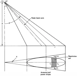
A forward looking radar (FLR) mounted on a platform at altitude h sends radio frequency (RF) pulses and scans around the vertical axis, resulting in a doughnut­ shaped coverage of the ground (see Fig. 8.7a). At any scan position, the area illu­ minated can be considered to be bounded by an elliptical contour, which is the radar antenna half-power gain pattern. The received signal at any scan position is the sum of the returns from all points in a resolution cell, that is, the region illuminated at distance r during the pulse interval. Therefore,

Jo!>o (r) f,fi (r)

vp (r, <!>) = up (r + s, <!> + 0')s ds d0'

-<t>o(r) 1 1

(r)

(8.5)

where <l>o _(r) is the angular width of the elliptical contour from its major axis, ₁₁ (r) and 12 (r) correspond to the inner and outer ground intercepts of radar pulse width around the point at radial distance r, and up (r, <!>) and vp (r, <!>) are the functions u (x, y) and

v (x, y ), respectively, expressed in polar coordinates. Figure 8. 7c shows the effect of scanning by a forward-looking radar. Note that the PSF associated with (8.5) is not shift invariant. (show!)

(b) object;

272

Antenna half· power ellipse

Cross section of radar beam (a) scanning geometry;

Figure 8.7 FLR imaging.

(c) FLR image (simulated).

d

10910 w _{Figure 8.8 Typical response of a photo­}

graphic film.

Detector and Recorder Models

The response of image detectors and recorders is generally nonlinear. For example, the response of photographic films, image scanners, and display devices can be written as

g = aw13 (8.6)

where a and 13 are device-dependent constants and w is the input variable. For photographic films, however, a more useful form of the model is (Fig. 8.8)

d = 'Y log10 w -do (8.7)

where 'Y is called the gamma of the film. Here w represents the incident light intensity and d is called the optical density. A film is called positive if it has negative 'Y. For 'Y =

-1, one obtains a linear model between w and the reflected or trans­ mitted light intensity, which is proportional to g � 10-d. For photoelectronic de­ vices, w represents the incident light intensity, and the output g is the scanning beam current. The quantity 13 is generally positive and around 0.75.

Noise Models

The general noise model of (8.3) is applicable in many situations. For example, in photoelectronic systems the noise in the electron beam current is often modeled as

TJ(X, y) = g (x, y) TJ1 (x, y) + TJ2 (x, y) (8.8) where g is obtained from (8.6) and TJi and TJz are zero-mean, mutually independent, Gaussian white noise fields. The signal-dependent term arises because the detection and recording processes involve random electron emission (or silver grain deposi­ tion in the case of films) having a Poisson distribution with a mean value of g. This distribution is approximated by the Gaussian distribution as a limiting case. Since the mean and variance of a Poisson distribution are equal, the signal-dependent term has a standard deviation

Vg

if it is assumed that TJi has unity variance. The

other term, TJ2, represents wideband thermal noise, which can be modeled as Gaus­ sian white noise.

In the case of films, there is no thermal noise and the noise model is

11(x, y) = g(x, y) 111 (x, y) (8.9)

where g now equals d, the optical density given by (8. 7). A more-accurate model for film grain noise takes the form

11(x, y) = e(g(x, y))" 111 (x, y) (8.10) where e is a normalization constant depending on the average film grain area and

{)-lies in the interval � to �- _J

The presence of the signal-dependent term in the noise model makes restora-tion algorithms particularly difficult. Often, in the funcrestora-tion f[g(w)], w is replaced by its spatial average µw, giving

11(x, Y) = f[ g (µw)]111 (x, y) + 112 (x, y) (8.11) which makes 11(x, y) a Gaussian white noise random field. If the detector is oper­ ating in its linear region, we obtain, for photoelectronic devices, a linear observa­ tion model of the form

v(x, y) = w (x, y) + v;:,,1 (x, y) + TJ2 (x, y) (8.12)

where we have set a = 1 in (8.6) without loss of generality. For photographic films (with 'Y = - 1), we obtain

v (x, y) = -log10 w + llTJ1 (x, y) -do (8.13)

where a is obtained by absorbing the various quantities in the noise model of (8.10).

The constant d0 has the effect of scaling w by a constant and can be ignored, giving v (x, y) = -log10 w + llTJ1 (x, y) (8.14)

where v (x, y) represents the observed optical density. The light intensity associated with v is given by

i(x, y) = 10-v(x,y)

= w(x, y)10-•"1Ji(x,y)

= w(x, y)n(x, y) (8.15)

where n � 10-•'11 now appears as multiplicative noise having a log-normal distribu­

tion.

A different type of noise that occurs in the coherent imaging of objects is called speckle noise. For low-resolution objects, it is multiplicative and occurs whenever the surface roughness of the object being imaged is of the order of the wavelength of the incident radiation. It is modeled as

v(x, y) = u(x, y)s(x, y) + 11(x, y) (8.16) where s (x, y), the speckle noise intensity, is a white noise random field with ex­ ponential distribution, that is,

exp

(:�)

, � :::O otherwise

Digital processing of images with speckle is discussed in section 8.13. Sampled Image Observation Models

(8. 17)

With uniform sampling the observation model of (8.1)-(8.3) can be reduced to a discrete approximation of the form

8.3 INVERSE AND WIENER FIL TERI NG Inverse Filter

Inverse filtering is the process of recovering the input of a system from its output. For example, in the absence of noise the inverse filter would be a system that

Inverse filters are useful for precorrecting an input signal in anticipation of the degradations caused by the system, such as correcting the nonlinearity of a display. Design of physically realizable inverse filters is difficult because they are often

u(m, n ) w(m, n)

h(m, n; k, l ) v(m, n)

System

Figure 8.9 Inverse filter.

Sec. 8.3 I nverse and Wiener Filtering

u(m, n ) h1( m, n; k, l )

I nverse filter

unstable. For example, for spatially invariant systems (8.23) can be written as

LL h1 (m - k', n - l')h (k', I') = B(m, n), V(m, n) (8.24) k',I' = -�

Fourier transforming both sides, we obtain _{H1 ( w17 w2)H(w17 w2)}

=

1 , which gives

H1 ( w17 w2) = _{H( Wi, Wz} 1 ₎ (8.25)

that is, the inverse filter frequency response is the reciprocal of the frequency response of the given system. However, H1 ( w17 w2) will not exist if H(w1, w2) has any zeros.

Pseudoinverse Filter

The pseu'doinverse filter is a stabilized version of the inverse filter. For a linear shift invariant system with frequency response H ( w17 w2), the pseudoinverse filter is defined as

H- (w,, w2) = w2)' H

+. O

0, H = O (8.26)

Here, H- ( w1, w2) is also called the generalized inverse of H ( w1, w2), in analogy with the definition of the generalized inverse of matrices. In practice, H- (w17 w2) is set to zero whenever IHI is less than a suitably chosen positive quantity E .

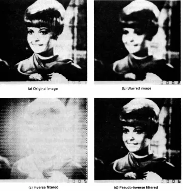
Example 8.3

Figure 8.10 shows a blurred image simulated digitally as the output of a noiseless linear system. Therefore, W(wi, w2) = H(wi, w2)U(wi , wz). The inverse filtered image is ob­ tained as 0 ( w1 w2)

�

W(w1, w2)1H(w1, w2). In the presence of additive noise, the in­ verse filter output can be written as

• W N N

U = + = U +

-H -H H (8.27)

where N(wi , w2) is the noise term. Even if N is small, NIH can assume large values resulting in amplification of noise in the filtered image. This is shown in Fig. 8. lOc, where the small amount of noise introduced by computer round-off errors has been amplified by the inverse filter. Pseudoinverse filtering reduces this effect (Fig. 8. lOd).

The Wiener Filter

The main limitation of inverse and pseudoinverse filtering is that these filters remain very sensitive to noise. Wiener filtering is a method of restoring images in the presence of blur as well as noise.

Let u(m, n) and v (m, n) be arbitrary, zero mean, random sequences. It is desired to obtain an estimate, u (m, n), of u(m, n) from v(m, n) such that the mean square error

a� = E{[u (m, n) -u (m, n)]2} (8.28)

(a) Original image (b) Blurred image

(c) Inverse filtered (d) Pseudo-inverse filtered

Figure 8.10 Inverse and pseudo-inverse filtered images.

is minimized. The best estimate Ct (m, n) is known to be the conditional mean of u (m, n) given {v (m, n), for every (m, n)}, that is,

Ct (m, n) = E[u(m, n)Jv (k, /), \f(k, /)] (8.29)

Equation (8.29), simple as it looks, is quite difficult to solve in general. This is because it is nonlinear, and the conditional probability density Puiv' required for solving (8.29) is difficult to calculate. Therefore, one generally settles for the best linear estimate of the form

u (m, n) =

LL

g(m, n ; k, t)v(k, t) (8.30)

k, I = - �

where the filter impulse response g(m, n ; k, I) is determined such that the mean square error of (8.28) is minimized. It is well known that if u (m, n) and v (m, n) are

jointly Gaussian sequences, then the solution of (8.29) is linear. Minimization of

(8.28) requires that the orthogonality condition

E[{u(m, n) - u (m, n)}v(m ', n ')] = 0, V(m, n), (m ', n ')

be satisfied. Using the definition of cross-correlation r0b (m, n ; k,

I) � E[a(m, n)b (k, /)]

correlation function of the observed image v (m, n) and its cross-correlation with the object u(rri, n) are known, then (8.33) can be solved in principle. Often, u(m, n) and v (m, n) can be assumed to be jointly stationary so that

rab (m, n ; m ', n ') = rab (m - m ', n - n ') (8.34)

for (a, b) = (u, u), (u, v), (v, v), and so on. This simplifies g(m, n; k, I) to a spatially invariant filter, denoted by g(m - k, n -1), and (8.33) reduces to

2:2: g(m - k, n - l)rvv (k, I) = ruv (m, n)

k, 1 = -"'

Taking Fourier transforms of both sides, and solving for G ( w" w2), we get G ( w,, Wz) = Suv ( WJ, Wz)S;;-v' ( W 1 , Wz)

(8.35)

(8.36)

where G, Suv' and Svv are the Fourier transforms of g, ruv, and rvv respectively. Equation (8.36) gives the Wiener filter frequency response and the filter equations become

v (m, n) is modeled by a linear observation system with additive noise, that is, v(m, n) = 2:2: h(m - k, n - l)u(k, I) + TJ(m, n) (8.39)

k, I = -�

where 11(m, n) is a stationary noise sequence uncorrelated with u(m, n) and which has the power spectral density S,,,,. Then

Svv (w,, Wz) = _{IH(w" w2)12 Suu (wi, w2) + S,,,, (wi, w2)}

(8.40)

This gives

(8.41)

which is also called the Fourier-Wiener filter. This filter is completely determined by the power spectra of the object and the noise and the frequency response of the imaging system. The mean square error can also be written as

CJ� =

Jr

_{S, (wi. W2) dw1 dw2} where S., the power spectrum density of the error, is

S, (wi, w2)

�

ll - GHl2 Suu + IGl2 STJTJ With G given by (8.41), this gives

Remarks

S = SuuST\T\ e

IHl2 Suu + ST\T\

(8.42a)

(8.42b)

(8.42c)

In general, the Wiener filter is not separable even if the PSF and the various covariance functions are. This means that two-dimensional Wiener filtering is not equivalent to row-by-row followed by column-by-column one-dimensional Wiener filtering.

Neither of the error fields, e(m, n) = u(m, n) - u(m, n), and e(m, n) �

v(m, n) - h (m, n) ® u(m, n), is white even if the observation noise TJ(m, n) is white.

Wiener Filter for Nonzero Mean Images. _{The foregoing development} requires that the observation model of (8.39) be zero mean. There is no loss of generality in this because if u(m, n) and TJ(m, n) are not zero mean, then from (8.39)

µv (m, n) = h (m, n) ® µu (m, n) + µTJ (m, n), µx

�

E[x] (8.43)

which gives the zero mean model

v (m, n) = h(m, n) ® u (m, n) + ii (m, n) (8.44)

where i � x -µx. In practice, µv can be estimated as the sample mean of the

observed image and the Wiener filter may be implemented on v (m, n). On the other

hand, if µu and µTl are known, then the Wiener filter becomes

= GV + IH21S S Mu - GMT\ uu + T]Tj

(8.45)

where M(wi, w2)

�

.:7{µ(m, n)} is the Fourier transform of the mean. Note that the

above filter allows spatially varying means for u(m, n) and TJ(m, n). Only the covar­

iance functions are required to be spatially invariant. The spatially varying mean may be estimated by local averaging of the image. In practice, this spatially varying filter can be quite effective. If µu and µTl are constants, then Mu and MT] are Dirac delta functions at 1;1 = 1;2 = 0. This means that a constant is added to the processed image which does not affect its dynamic range and hence its display.

Phase of the Wiener Filter. Equation (8.41) can be written as

G = jGje i0a

jGj = _{IHl2 Suu} IHISuu

+ 51111

0G = 0G (wi, _W2) = 0w = -0H = 0H-1

(8.46)

that is, the phase of the Wiener filter is equal to the phase of the inverse filter (in the frequency domain). Therefore, the Wiener filter or, equivalently, the mean square criterion of (8.28), does not compensate for phase distortions due to noise in the observations.

Wiener Smoothing Filter. _{In the absence of any blur, H} = 1 _{and the} Wiener filter becomes

I Suu Snr

G H= 1 = s + s s 1 uu 1111 nr + (8.47) where Sn, � SuulS1111 defines the signal-to-noise ratio at the frequencies (w17 w2). This is also called the (Wiener) smoothing filter. It is a zero-phase filter that depends only

_,,

w , _____ "

(a) Noise smoothing (H = 1 )

w , _

(b) Deblurring

Figure 8.11 Wiener filter characteristics.

on the signal-to-noise ratio Snr· For frequencies where Sn, � 1 , G becomes nearly equal to unity which means that all these frequency components are in the passband. When Sn, � 1 , G = Sn, ; that is, all frequency components where Sn, � 1 , are attenuated in proportion to their signal-to-noise ratio. For images, Sn, is usually high at lower spatial frequencies. Therefore, the noise smoothing filter is a low-pass filter (see Fig. 8. lla).

Relation with Inverse Filtering. _{In the absence of noise, we set} S,,,, ₌ 0 _and

the Wiener filter reduces to

(8.48) which is the inverse filter. On the other hand, taking the limit s,,,,�o, we obtain

lim G =

1�'

H

=I= O

= H-s��-. o

0, H = 0 (8.49)

which is the pseudoinverse filter. Since the blurring process is usually a low-pass filter, the Wiener filter acts as a high-pass filter at low levels of noise.

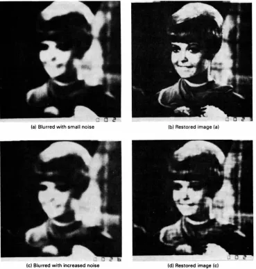
Interpretation of Wiener Filter Frequency Response. _{When both noise} and blur are present, the Wiener filter achieves a compromise between the low-pass noise smoothing filter and the high-pass inverse filter resulting in a band-pass filter (see Fig. 8. llb ). Figure 8.12 shows Wiener filtering results for noisy blurred images. Observe that the deblurring effect of the Wiener filter diminishes rapidly as the noise level increases.

Wiener Filter for Diffraction Limited Systems. _{The Wiener filter for the} continuous observation model, analogous to (8.39)

v (x, y) =

Jr

h(x - x ', y - y ')u(x', y')dx 'dy ' + TJ(X, y) (8.50) is given by

(8.51) For a diffraction limited system, H(�i, �2) will be zero outside a region, say 9l , in the frequency plane. From (8.51), G will also be zero outside 9l . Thus, the Wiener filter cannot resolve beyond the diffraction limit.

Wiener Filter Digital Implementation. _{The impulse response of the} Wiener filter is given by

(8.52)

(a) Blurred with small noise (b) Restored image (a)

(c) Blurred with increased noise (d) Restored image (c)

Figure 8.12 Wiener filtering of noisy blurred images.

This integral can be computed approximately on a uniform N x N grid as

N/2 - 1

g (m, n) =

-1z

_N

LL

G (k, l)w-(mk + nfJ, _ N :=; m, n :=; N - l (8.53)

(k, f) =

-N/2

2 2

where G (k, _/)

�

G (2Tik/N, 27rl/N), W

�

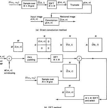
exp(-j2Ti/N). The preceding series can be calculated via the two-dimensional FFf from which we can approximate g(m, n) by g (m, n) over the N x N grid defined above. Outside this grid g(m, n) is assumed to be zero. Sometimes the region of support of g(m, n) is much smaller than the N x N grid. Then the convolution of g (m, n) with v (m, n) could be implemented directly in the spatial domain. Modern image processing systems provide such a facility in hardware allowing high-speed implementation. Figure 8. 13a shows this algorithm.

Sample over G(k, I) _. IDFT g(m, n)c

Figure 8.13 Digital implementations of the Wiener filter.

Alternatively, the Wiener filter can be implemented in the DFf domain as shown in Fig. 8. 13b. Now the frequency response is sampled as G _{(k, /) and is}

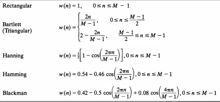
multiplied by the DFf of the zero-padded, windowed observations. An appropriate region of the inverse DFf then gives the restored image. This is simply an imple­ mentation of the convolution of g(m, n) with windowed v (m, n) via the DFf. The windowing operation is useful when an infinite sequence is replaced by a finite sequence in convolution of two sequences. Two-dimensional windows are often taken to be separable product of one-dimensional windows as

w(m, n) = w1 (m)w2 (n) (8.54)

where w1 (m) and w2 (n) are one-dimensional windows (see Table 8.2). For images of size 256 x 256 or larger, the rectangular window has been found to be appropriate. For smaller size images, other windows are more useful. If the image size is large and the filter g(m, n) can be approximated by a small size array, then their con­ volution can be realized by filtering the image in small, overlapping blocks and summing the outputs of the block filters [9].

TABLE 8.2 One-Dimensional Windows w(n ) for 0

s

n

s

M

-

1

8.4 FINITE IMPULSE RESPONSE (FIR) WIENER FILTERS

Theoretically, the Wiener filter has an infinite impulse response which requires working with large size DFfs. However, the effective response of these filters is often much smaller than the object size. Therefore, optimum FIR filters could achieve the performance of IIR filters but with lower computational complexity.

Filter Design

An FIR Wiener filter can be implemented as a convolution of the form

u (m, n) = LL g(i,j)v(m - i, n - j)

(i,J) E W

W = {-M $ i, j $ M}

(8.55) (8.56) where g (i, j) are the optimal filter weights that minimize the mean square error E[{u(m, n) -u (m, n)}2]. The associated orthogonality condition

E[{u(m, n) -u (m, n)}v(m - k, n - l)] = 0, reduces to a set of (2M + 1)2 simultaneous equations

ruv (k, /) - LL g (i, j)rvv (k - i, / - j) = 0,

284 Image Filtering and Restoration

(8.59) (8.60)

ruv (k, I) = h (k, I) * ruu (k, I) = 2:2: h (i, j)ruu (i + k, j + /)

In matrix form this becomes a block Toeplitz system

[:;I+ gi]

� = �UV (8.64) Fourier transforms of IH(wi, w2)12 and Suu (wi, w2)H* (wi. w2), respectively.

When there is no blur (that is, H = 1), h (k, /) = 8(k, /), ruv (k, l) = ruu (k, l) and the resulting filter is the optimum FIR smoothing filter.

The size of the FIR Wiener filter grows with the amount of blur and the additive noise. Experimental results have shown that FIR Wiener filters of sizes up to 15 x 15 can be quite satisfactory in a variety of cases with different levels of blur and noise. In the special case of no blur, (8.63) becomes

[

:;

S(k, /) + r0 (k,

/)]

© g (k, I) = r0 (k, /), (k, /) E W (8.65) From this, it is seen that as the SNR = 1J2/1J;� oo, the filter response g(k, l)� B(k, /), that is, the FIR filter support goes down to one pixel. O n the other hand, if SNR = 0, g (k, /) = ( 1J 2/1J';)r0 (k, I). This means the filter support would effectively be the same as the region outside of which the image correlations are negligible. For images with r0 (k, I) = 0. + (!., this region happens to be of size 32 x 32.

In general, as IJ';� 0, g(m, n) becomes the optimum FIR inverse filter. As M � oo, g (m, n) would converge to the pseudoinverse filter.

(a) Blurred image with no noise (b) Restored by optimal 9 x 9 FIR filter

(c) Blurred image with small additive noise (d) Restored by 9 x 9 optimal FIR filter

Figure 8.14 FIR Wiener filtering of blurred images.

Example 8.4

286

Figure 8.14 shows examples of FIR Wiener filtering of images blurred by the Gaussian PSF

h (m, n) = exp{-a(m 2 + _n 2_)}, a > O (8.66) and modeled by the covariance function r(m, n) = If a = 0, and h (m, n) is restricted to a finite region, say -p :5, m, n :5, p, then the h(m, n) defined above can be used to model aberrations in a lens with finite aperture. Figs. 8.15 and 8.16 show examples of FIR Wiener filtering of blurred images that were intentionally misfocused by the digitizing camera.

(a) Digitized image (b) FIR filtered

(c) Digitized image (d) FIR filtered Figure 8.15 FIR Wiener filtering of improperly digitized images.

Spatially Varying FIR Filters

The local structure and the ease of implementation of the FIR filters makes them attractive candidates for the restoration of nonstationary images blurred by spatially varying PSFs. A simple but effective nonstationary model for images is one that has spatially varying mean and variance functions and shift-invariant correlations, that is,

Sec. 8.4

E[u (m, n)] = µ(m, n)

l

E[{u(m, n) - µ(m, n)} {u(m -k, n -l) - µ(m - k, n - l)}]

= cr2 (m, n)r0 (k, l)

Finite I m pu lse Response (FIR) Wiener Filters

(8.67)

(a) Digitized image (b) FIR filtered

PLASMA CARBURl lllG

VI/ 0 10£

(c) Digitized image (d) FIR filtered

Figure 8.16 FIR Wiener filtering of improperly digitized images.

where r0 (0, 0) = ·1. If the effective width of the PSF is less than or equal to W, and h, µ, and cr 2 are slowly varying, then the spatially varying estimate can be shown to be

given by (see Problem 8.10)

u (m, n) = LL

gm,n(i,j)v(m -i,

n

-j)

(8.68)

(i, j) E

W

gm,n (i, j) � 8m,n (i, j)

+ _(2M l_{+ l)2}

[

1

-(k

��

_Wgm,n

(k,

l)]

(8.69) where

gm, n (i, j)

is the solution of (8.64) with cr 2 = cr 2 (m, n). The quantity cr 2 (m, n)

can be estimated from the observation model. The second term in (8.69) adds a

constant with respect to (i, j) to the FIR filter which is equivalent to adding to the estimate a quantity proportional to the local average of the observations.

Example 8.5

Consider the case of noisy images with no blur. Figures 8.17 and 8. 18 show noisy images with SNR = 10 dB and their Wiener filter estimates. A spatially varying FIR Wiener filter called Optmask was designed using CJ' 2 (m, n) = CJ'� (m, n) - CJ' 2, where CJ'� (m, n) was estimated as the local variance of the pixels in the neighborhood of (m, n ). The size of the Optmask window W has changed from resion to region such that

the output SNR was nearly constant [8] . This criterion gives a uniform visual quality to the filtered image, resulting in a more favorable appearance. The images,obtained by

(a) Noisy (SNR = 1 0dB) (b) Wiener

(c) Cosar (d) Optmask

Figure 8.17 Noisy image (SNR = 10 dB) and restored images.

(a) Noisy (SNR = 1 0dB) (b) Wiener

(c) Cesar (d) Optmask

Figure 8.18 Noisy image (SNR = 10 dB) and restored images.

the Casar filter are based on a spatially varying AR model, which is discussed in Section 8. 12. Comparison of the spatially adaptive FIR filter output with the con­ ventional Wiener filter shows a significant improvement. The comparison appears much more dramatic on a good quality CRT display unit compared to the pictures printed in this text.

8.5 OTHER FOURIER DOMAIN FILTERS

The Wiener filter of (8.41) motivates the use of other Fourier domain filters as discussed below.

Geometric Mean Filter

This filter is the geometric mean of the pseudoinverse and the Wiener filters, that is,

(

s

H* )1-s

Gs= (H-Y

Suu + S,,,, '

For s = !, this becomes

O :s; s :s; l

G112

= _S

)112 IHH-1112

exp{-j0H}

uu + ,,,,

(8.70)

(8.71) where _{0H (wi, w2)} is the phase of H(wi, w

2

). Unlike the Wiener filter, the power spectral density of the output of this filter is identical to that of the object when

H-=/=

0. As S,,,,� 0, this filter also becomes the pseudoinverse filter (see Problem 8.11).

Nonlinear Filters

These filters are of the form

(8. 72) where

G

(x, wi, w2) is a nonlinear function of x. Digital implementation of such nonlinear filters is quite easy. A simple nonlinear filter, called the root-filter, is defined as

(8.73) Depending on the value of a _{this could be a low-pass, a high-pass, or a band-pass} filter. For values of a � 1, _{it acts as a high-pass filter (Fig.} 8.19) for typical images

(a) a = 0.8 (b) a = 0.6

Figure 8.19 Root filtering of FLR image of Fig. 8.7c.

(having small energy at high spatial frequencies) because the samples of low amplitudes of V(wi. wi) are enhanced relative to the high-amplitude samples. For a � 1 , the large-magnitude samples are amplified relative to the low-magnitude ones, giving a low-pass-filter effect_ for typical images. Another useful nonlinear filter is the complex logarithm of the observations

O ( w w i , i ) =

{

{logiVl}exp{j0v}, IVI O, 2:: E .

otherwise (8.74)

where E is some preselected small positive number. The sequence u (m, n) is also

called the cepstrum of v (m, n ). (Also see Section 7 .5.)

8.6 FILTERING USING IMAGE TRANSFORMS Wiener Filtering

Consider the zero mean image observation model

v (m, n) = L L h (m, n ; i, j)u(i, j) + TJ(m, n),

i j (8.75)

0 :s; m :s; N, - 1, 0 :s; n :s; Ni - 1

Assuming the object u(m, n) is of size M1 x Mi the preceding equation can be written as (see Chapter 2)

(8.76)

where o- and ,,, are N1 Ni x 1, a-is M1 Mi x 1 and .9'C is a block matrix. The best

linear estimate

a, = /j' 0-that minimizes the average mean square error

a� = _M,l_{MiE[(u- - iu)}T(u- - iu)]

is obtained by the orthogonality relation

E[(u- - iu)o-T] = 0 This gives the Wiener filter as an M1 Mi x N1 Ni matrix

/J' = E [ u-o-T]{ E [ o-o-TU-l = Yl9C'[ ,9'CytgCT + Yint 1

(8.77)

(8.78)

(8.79)

(8.80)

where Yi and Yin are the covariance matrices of a-and ,,,, respectively, which are assumed to be uncorrelated, that is,

(8.81) The resulting error is found to be

1 a� =

MiMi Tr[(I - /J'.9C)Yl) (8. 82)

Assuming {Jl and f7l" to be positive definite, (8.80) _{can be written via the ABCD} lemma for inversion of a matrix A -BCD (see Table 2.6) _as

(8.83) For the stationary observation model where the PSF is spatially invariant, the object is a stationary random field, and the noise is white with zero mean and variance er�,

the Wiener filter becomes

(8.84)

where {Jl and .'TC are doubly block Toeplitz matrices.

In the case of no blur, .'TC= I, and /7 becomes the optimum noise smoothing filter

(8.85)

Remarks

If the noise power goes to zero, then the Wiener filter becomes the pseudoinverse of 9'C (see Section 8.9), _{that is,} the object and noise covariance functions are separable. However, the pseudo­ inverse filter 17-is separable if 9Z and .'TC are.

The Wiener filter for nonzero mean random variables u and ,,, becomes

(8.87) This form of the filter is useful only when the mean of the object and/or the noise are spatially varying.

Generalized Wiener Filtering

The size of the filter matrix /7 becomes quite large even when the arrays u(m, n)

and v(m, n) are small. For example, for 16 x 16 arrays, /7 is 256 x 256. Moreover,

to calculate 17, a matrix of size M1 M2 x M1 M2 or N1 N2 x N1 N2 has to be inverted. Generalized Wiener filtering gives an efficient method of approximately imple­ menting the Wiener filter using fast unitary transforms. For instance, using (8.84) _in (8.77) _{and defining}

we can write

1; = Jt*T[Jt�*7).A'[.9'CT 0

])

� Jt*T ffiw

Sec. 8.6 Filtering Using Image Transforms

(8.88)

(8.89)

where .A is a unitary matrix,

ftJ

�

.A!lJ.A*r, ro

�

.A[.9CT u ]. This equation sug­

gests the implementation of Fig. 8.20 and is called generalized Wiener filtering. For stationary observation models, gcr u is a convolution operation and ?tJ turns out to

be nearly diagonal for many unitary transforms. Therefore, approximating

6. -

-W-= !lJw-= [Diag!lJ)w- (8.90)

and mapping w- and W-_{back into N1} x _{N2 arrays, we get}

w (k,

l)

= p (k,

l)w

(k,

l)

(8.91) where p (k,

l)

come from the diagonal elements of

ftJ.

Figure 8.20 shows the imple­ mentation of generalized Wiener filtering when ftJ is approximated by its diagonal. Now, if .A is a fast transform requiring O (N1 N2 log N1 N2) operations for trans­ forming an N1 x _{N2 array, the total number of operations are reduced from}

0 (M? Mn to 0 (M1 M2 log M1 M2). For 16 x 16 arrays, this means a reduction from 0 (224) to 0 (211). Among the various fast transforms, the cosine and sine transforms have been found useful for generalized Wiener filtering of images [12, 13).

The generalized Wiener filter implementation of Fig. 8.20 is exact when .A diagonalizes !lJ. However, this implementation is impractical because this diagonal­ izing transform is generally not a fast transform. For a fast transform .A, the diagonal elements of !lJ may be approximated as follows

Diag{

ftJ}

= Diag{.A(.9Cr gc + cr� .9'l-1r1.A*7}

= (Diag{.A.9Cr .9C.A* 1} + cr�(Diag{Jt.g't.A*7}t1r1

where we have approximated Diag{.A.9'l-1 .A*7} by (Diag{.A.9'l.A*7}r1• This gives p (k,

l)

=

(h2(k, /) + 1cr� l.Y(k, /)) (8.92) where h2(k,

l)

and .Y(k, /) are the elements on the diagonal of ,Ager .9CJt.*T and Jt.g'l,A*r, respectively. Note that .Y(k, /) are the mean square values of the trans­ form coefficients, that is, if iD � .Aa, then .Y(k,

l)

= E[lu (k, /)12) .

v(m, n)

h(-m, -n)

294

(a) Wiener filter in .�·transform domain

2-D image

Figure 8.20 Generalized Wiener filtering.

2-D inverse transform

Image Filtering and Restoration

u(m, n)

Filtering by Fast Decompositions [13]

For narrow PSFs and stationary observation

decompose the filter gain matrix Y as models, it is often possible to

Y = Yo + Ub, Yo � ffio!TCT, (8.93)

where .00 can be diagonalized by a fast transform and ffib is sparse and of low rank. Hence, the filter equation can be written as

A .:i ' O ' b ( ₎

IV = 0-= 0 0- 0-= IV + IV 8.94 When JiJ0 � ut!lJ0ut* T is diagonal for some fast unitary transform ._A,, the com­ ponent U-0 can be written as

u,0 = ffio!TCT 0-=ut*T[utffiout*1ut[!TCT o-] = ._A,*T JiJo _fO (8.95) and can be implemented as an exact generalized Wiener filter. The other compo­ nent, U,b, generally requires performing operations on only a few boundary values of

gcT o-. The number of operations required for calculating U,b depends on the width of the PSF and the image correlation model. Usually these require fewer operations than in the direct computation of iv from Y. Therefore, the overall filter can be implemented quite efficiently. If the image size is large compared to the width of the PSF, the boundary response can be ignored. Then, Y is approximately Yo, which can be implemented via its diagonalizing fast transform [13].

8.7 SMOOTHING SPLINES AND INTERPOLATION [15-17]

Smoothing splines are curves used to estimate a continuous function from its sample values available on a grid. In image processing, spline functions are useful for magnification and noise smoothing. Typically, pixels in each horizontal scan line are first fit by smoothing splines and then finely sampled to achieve a desired magnifica­ tion in the horizontal direction. The same procedure is then repeated along the vertical direction. Thus the image is smoothed and interpolated by a separable function.

Let

{y;,

0 ::5 i ::5 N} be a given set of (N

+

1) observations of a continuous function f(x) sampled uniformly (this is only a convenient assumption) such that

X; = x0 + ih, h > 0 and

(8.96) where n(x) represents the errors (or noise) in the observation process. Smoothing splines fit a smooth function g (x) through the available set of observations such that its "roughness," measured by the energy in the second derivatives (that is, f[d2g(x)ldx2]2dx), over [x0,xN] is minimized. Simultaneously, the least squares error at the observation points is restricted, that is, for g;

�

g(x;),

Sec. 8.7

F

�

i

�)

g; ::5

s

(8.97)

For S = 0, this means an absolute fit through the observation points is required. Typically, CJ� is the mean square value of the noise and S is chosen to lie in the range

(N

+ 1) ± + 1), which is also called the confidence interval of S. The minimi­ zation problem has two solutions:

1. When S is sufficiently large, the constraint of (8.97) is satisfied by a straight­ line fit

(8.98)

N

where µ denotes sample average, for instance, µx �

(�0

x}(N

+ 1), and so on. 2. The constraint in (8.97) is tight, so only the equality constraint can be satis­

fied. The solution becomes a set of piecewise continuous third-order polynomials called cubic splines, given by

X; :5 X < X; + 1 (8.99)

The coefficients of these spline functions are obtained by solving [P + >..Q]c = >..v,

CJ2

a = y - -nLc _>..

d· = I C; + 1 - C; 3h 1

.-h2d.

I h c, l l 0 ::s i ::s N-l

(8.100)

where a and y are

(N

+ 1) x 1 vectors of the elements {a;, 0 ::::; i ::::;

N},

{y;, 0 :5 i :5

N},

respectively, and c is the (N -1) x 1 vector of elements [c;, 1 s i s

N

- l]. The matrices Q and L are, respectively,

(N

-1) x

(N

- 1) tridiagonal Toeplitz and

(N

+ 1) x

(N

-1) lower triangular Toeplitz, namely,

4

and P � CJ� LTL. The parameter >.. is such that the equality constraint

F(>..) � Ila -2yll2 = vT APAv = S CJ n

296 Image Filtering and Restoration

(8.101)

(8.102)

where A � [P + A.Qi-', is satisfied. The nonlinear equation F(X.) = S is solved y based on appropriate autocorrelation models (see Problem 8.15).

The special case S = 0 gives what are called the interpolating splines, where the splines must pass through the given data points.

Example 8.6 reduced to least squares minimization problems. In this section we consider such problems in the context of image restoration.

Constrained Least Squares Restoration

Consider the spatially invariant image observation model of (8.39). The constrained least squares restoration filter output it (m, n), which is an estimate of u(m, n), minimizes a quantity

J

�

llq(m, n) 0 it (m, n)ll2 (8.104)

subject to the constraint implies smoothing of high frequencies or rough edges. Using the Parseval relation this implies minimization of

subject to

A

2 2 llV(wi, w2) - H(wi, w2)U(wi, w2)ll ::5 E

The solution obtained via the Lagrange multiplier method gives U(w1, w2) = Gt. (w" w2)V(wi, w2)

The Lagrange multiplier 'Y is determined such that 0 satisfies the equality in

(8.108) subject to (8. 109) and (8.110). This yields a nonlinear equation for 'Y: ll.

_.::L

_ff"

IQ

14

IVl2 _ 2 _

f('Y) = 47T2_,, (IHl2+'YIQl2)2dw,dw2 E - 0 (8.111)

In least squares filtering, q (m, n) is commonly chosen as a finite difference approxi­ mation of the Laplacian operator a2Jax2 + a2Jay2• For example, on a square grid with spacing ll.x = ll.y = 1 , and a = � below, one obtains

q (m, n) � -S(m, n) + a[S(m - 1, n) + S(m + 1, n)

+ S(m, n -1) + S(m, n + 1)]

which gives Q ( wi, w2) = - 1 + 2a cos w1 + 2a cos w2.

Remarks

For the vector image model problem,

o- = 9'Cu-+ n,

m_in IWaf,

"

where $ is a given matrix, the least squares filter is obtained by solving

U _{= ('Y4'T 4' + ,gcT} 9'C)-I ,gcT

In the absence of blur, one obtains the least squares smoothing filter

U, =

(

"1

4

T

4+ It1 0-

(8.116)

This becomes the two-dimensional version of the smoothing spline solution if$ is obtained from the discrete Laplacian operator of

(8.112).

A _{recursive solution of} this problem is considered in

[32].

Comparison of

(8.110)

and

(8.116)

with

(8.41)

and

(8.84),

respectively, shows that the least squares filter is in the class of Wiener filters. For example, if we specify

ST]T]

�"I

and Suu

=

lllQ 12,

then the two filters are identical. In fact, specifying g (m, n) is equivalent to modeling the object by a random field whose power spectral density function is

1/IQ 12

(see Problem

8.17).

8.9 GENERALIZED INVERSE, SVD, AND ITERATIVE METHODS

The foregoing least squares and mean square restoration filters can also be realized by direct minimization of their quadratic cost functionals. Such direct minimization techniques are most useful when little is known about the statistical properties of the observed image data and when the PSF is spatially variant. Consider the image observation model

v = Hu

(8.117)

where v and u are vectors of appropriate dimensions and H is a rectangular (say M x N) PSF matrix. The unconstrained least squares estimate u minimizes the norm

J = llv - Hull2

The Pseudoinverse

A solution vector u that minimizes

(8.118)

must satisfy

HTHil = HTv

If HT H is nonsingular, this gives

u = u-v,

(8.118)

(8.119)

(8.120)

as the unique least squares solution. u- is called the pseudoinverse of H. This pseudoinverse has the interesting property

u-u = I

(8.121)

Note, however, that uu- =f:.

I.

If H is M x N, then u-is N x M. A necessary condition for HTH to be nonsingular is that M � N and the rank of H should be N.

If M < N _{and the rank of} H _is M, _{then the pseudoinverse of} H _{is defined as a matrix}

H-, which satisfies

uu- = 1

(8.122)

In this case, H-is not unique. One solution is

u- = ur(uur(1•

(8.123)

In general, whenever the rank of

H

is

r

< N,

(8.119)

_{does not have a unique}

solution. Additional constraints on u are then necessary to make it unique.

Minimum Norm Least Squares (MNLS) Solution and the Generalized Inverse

A vector

u+

that has the minimum norm llu!l2 among all the solutions of

(8.119)

is called the MNLS (minimum norm least squares) solution. Thus

u+ =

min{llu!l2;

uruu

=

ur v}

(8.124)

,;

Clearly, if rank

[HrH] =

N, then

u+ =

u is the least squares solution. Using the singular value expansion of

H,

it can be shown that the transformation between

v

and

u+

is linear and unique and is given by

(8.125)

The matrix

u+

is called the

generalized inverse

of

H.

If the M x N matrix

H

has the SVD expansion [see

(5.188)]

(8.126a)

m=I

then,

u+

is an N x M matrix with an SVD expansion

(8.126b)

m=I

where

cf>m

and

"1m

are, respectively, the eigenvectors of

uru

and

uur

correspond­ ing to the singular values

{A.m, 1

:s m :s

r }.

Using

(8.126b

), it can be shown

u+

satisfies the following relations:

1.

u+ = (uru)-1 ur,

_if

r =

_N

2.

u+ = Hr (HHT(1,

if

r =

M

3.

uu+ = (uu+r

4.

u+u = (u+u)r

s.

uu+u = u

6.

u+uur= ur

The first two relations show that

u+

is a pseudoinverse if

r

= N or M. The

MNLS solution is

r

u+

=

L

A.;;,112 cf>m «;, v

(8.127)

m= I

This method is quite general and is applicable to arbitrary PSFs. The major difficulty is computational because it requires calculation of

lfik

and

cf>k

for large

matrices. For example, for M

=

N =

256, H

is

65,536

x

65,536.

For images with separable PSF, that is, V =

H1 UH2,

the generalized inverse is also separable, giving u+

= Ht vm.

One-Step Gradient Methods

When the ultimate aim is to obtain the restored solution

u+,

rather than the explicit pseudoinverse

H+,

then iterative gradient methods are useful. One-step gradient algorithms are of the form

u0= 0

(8.128)

(8.129)

where u" and g" are, respectively, the trial solution and the gradient of J at iteration step n and U'n is a scalar quantity. For the interval

0

s U'n

< 2/X.max (HTH), U

n con­ verges to the MNLS solution

u+

as n � oo. If U'n is chosen to be a constant, then its optimum value for fastest convergence is given by

[22]

2

U'opt

= [Amax (HTH) +Amin (HTH)]

(8.130)

For a highly ill conditioned matrix

HrH,

the condition number,

Amax IX.min

is large. Then CTopt is close to its upper bound,

2/X.max

and the error at iteration n, for U'n = CJ",

obeys

(8.131)

This implies that lien II is proportional to lien - 1 11, that is, the convergence is linear and can be very slow, because CJ" is bounded from above. To improve the speed of

convergence, CT is optimized at each iteration, which yields the steepest descent algorithm, with

(8.132)

However, even this may not significantly help in speeding up the convergence when the condition number of A is high.

Van Cittert Filter

[4]

From

(8.128)

and

(8.129),

the solution at iteration n

=

i, with U'n

= CT

can be written

as

where

G;

is a power series:

U;+1 = G;v,

i

2

O< CJ"<-

_Amax

G; =

(J' L

(I

-

CJ"HTH)kHT

k�O

Sec. 8.9 Generalized Inverse, SVD, and Iterative Methods

(8.133)

v(m, n)

This is called the Van Cittert filter. Physically it represents passing the modified observation vector rrHT v through i stages of identical filters and summing their outputs (Fig. 8.21). For a spatially invariant PSF, this requires first passing the observed image v (m, n) through a filter whose frequency response is rrH* ( w i . w2)

and then through i stages of identical filters, each having the frequency response 1 -rrlH ( Wi. w2)

1

2.

One advantage of this method is that the region of support of each filter stage is only twice (in each dimension) that of the PSF. Therefore, if the PSF is not too broad, each filter stage can be conveniently implemented by an FIR filter. This can be attractive for real-time pipeline implementations.

The Conjugate Gradient Method [22-24]

The conjugate gradient method is based on finding conjugate directions, which are vectors d; =F O, such that

i 4=

j,

0 :=::;

i, j

:=::; N -1 (8. 134)

When A is positive definite, such a set of vectors exists and forms a basis in the N-dimensional vector space. In terms of this basis, the solution can be written as

N - 1

u+ = 2: a; d; (8. 135)

i = O

The scalars a; and vectors d; can be calculated conveniently via the recursions

Ll in dn

Cl'.n - d�Ad/ - --- Uo Ll = 0

,:l in Adn - 1 ,:l

dn = -gn + l3n - 1 dn - 1' l3n - 1 = T , do = -go

dn - 1 Adn - 1

gn = -HT V + Aun = gn - 1 + Cl'.n -1 Adn - 1, go � -HT V

(8. 136)

In this algorithm, the direction vectors dn are conjugate and a" minimizes J,

not only along the nth direction but also over the subspace generated by

d0, di. . . . , dn -l · Hence, the minimum is achieved in at most N steps, and the method is better than the one-step gradient method at each iteration. For image restoration problems where N is a large number, one need not run the algorithm to completion since large reductions in error are achieved in the first few steps. When rank H is r

<

N, then it is sufficient to run the algorithm up to n = r -1 and u,� u+ .

;J;(m, n)

1 · · · - · · · i

Figure 8.21 Van Cittert filter.

The major computation at each step requires the single matrix-vector product

Adn. All other vector operations require only N multiplications. If the PSF is narrow compared to the image size, we can make use of the sparseness 0f A and all the operations can be carried out quickly and efficiently.

Example 8.7

Consider the solution of

This gives

A = HTH = [6 7]

_{7 14}

whose eigenvalues are A.1

= 10

+ \/65 and A.2

= 10

-\/65. Since

A

is nonsingular,

H+ = A-1HT= .l [ 14

-1

][

1

2

1

]

_{= .l}

[

o

21 -7]

35

-7 6 2

₁

3

₃₅

5 -8

_{1 1}

This gives

+

= H+ = .l[21] = [0.600]

u _{v 35}

22 0.628

and

llv -

Hu+ll2 = 1.02857

For the one-step gradient algorithm, we get

a = aopt = fo = O.l

and

After

12

iterations, we get

[0.685]

gll =

1.253 '

The steepest descent algorithm gives

[0.8]

U1

= 1.3 ,

[0.555]

u12 = 0.581 '

11 = 9.46

112 = 1.102

[0.5992]

u3

= 0.6290 '

13

= 1.02857.

The conjugate gradient algorithm converges in two steps, as expected, giving _u2

=

u+ . Both conjugate gradient and steepest descent are much faster than the one-step gradient algorithm.

Separable Point Spread Functions

If the two-dimensional point spread function is separable, then the generalized inverse is also separable. Writing V = _{H1 UHI,} we can rederive the various iterative

algorithms. For example, the matrix form of the conjugate gradient algorithm becomes

(8.137)

Gn = Gn

-I +

O'.n

-I A1

Dn

-I Az,

Do = Go =

H{VH2

where A1 � H{Hi, A2 = H�H2 and (X, Y) � Lm LnX(m, n)y(m, n). This algorithm

has been found useful for restoration of images blurred by spatially variant PSFs

[24].

8.10 RECURSIVE FILTERING FOR STATE VARIABLE SYSTEMS

Recursive filters realize an infinite impulse response with finite memory and are particularly useful for spatially varying restoration problems. In this section we con­ sider the Kalman filtering technique, which is of fundamental importance in linear estimation theory.

Kalman Filtering

[25, 26]

Consider a state variable system

n =

0

_{, 1 , . . .}

(8.138)

E[Xoxb)

= R0,

where

Xn, En, Zn

are m x 1 , p x 1 , and q x 1 vectors, respectively, all being Gaus­ sian, zero mean, random sequences. R0 is the covariance matrix of the initial state vector

Xo,

which is assumed to be uncorrelated with Eo . Suppose

Zn

is observed in the presence of additive white Gaussian noise as

n � O, !,

... l

_(8.139)

where

Ttn

and

En

are uncorrelated sequences. We define

Sn. gn.

and Xn as the best mean square estimates of the state variable

Xn

when the observations are available up to n -1 , n, and N > n, respectively. Earlier, we have seen that mean square estimation of a sequence x(n) from observations y(n

)

,

0

s n s N, gives us the Wiener filter. In this filter the entire estimated sequence is calculated from all the observations simultaneously [see

(8.77)].

Kalman filtering theory gives recursive realizations of these estimates as the observation data arrives sequentially. This reduces the computational complexity of the Wiener filter calculations, especially when the state variable model is time varying. However, Kalman filtering requires a stochastic model of the quantity to be estimated (that is, object) in the form of

(8. 138), whereas Wiener filtering is totally based on the knowledge of the auto­ correlation of the observations and their cross-correlation with the object (see

(8.80)]. The sequence vn is called the innovations process. It represents the new information obtained when the observation sample Yn arrives. It can be shown (25, 26] that Vn is a zero mean white noise sequence with covariances Qn, that is,

(8.142)

The nonlinear equation in (8. 141) is called the Riccati equation, where Rn represents the covariance of the prediction error en � Xn - sn, which is also a white sequence:

(8.143)

The m x q matrix Gn is called the Kalman gain. Note that Rn, Gn, and Qn depend only on the state variable model parameters and not on the data. Examining (8. 140)

and Fig. 8.22 we see that the model structure of sn is recursive and is similar to the state variable model. The predictor equation can also be written as

Sn + ! =

_

An Sn + Gn q�1 Vn

l

(8.144)

Yn - Cn Sn + Vn

which is another state variable realization of the output sequence Yn from a white sequence Vn of covariances Qn· This is called the innovations representation and is

useful because it is causally invertible, that is, given the system output Yn, one can find the input sequence Vn according to (8. 140). Such representations have applica­ tion in designing predictive coders for noisy data (see (6] of Chapter 11).

Online filter. The online filter is the best estimate of the current state based on all the observations received currently, that is,

gn � E(xnlYn·, 0 :s n ' :s n

]

(8. 145)

This estimate simply updates the predicted value sn by the new information vn with a gain factor Rn C�q�1 to obtain the most current estimate. From (8. 140), we now see that

(8. 146)

State model

Unit _Xn delay

z-1

(a) State variable model

(b) One step predictor

Observation model

Unit _sn

delay z-1

filter

sn predictor

�::

(c) Online filter

Figure 8.22 Kalman filtering.

Therefore, Kalman filtering can be thought of as having two steps (Fig. 8.22c). The first step is to update the previous prediction by the innovations. The next step is to predict from the latest update.

Fixed-interval smoother (Wiener filter). _{Suppose the observations are} available over the full interval [O, N]. Then, by definition,

Xn = E

[

xnlYn·,

0

::5 n I ::5 N]

is the Wiener filter for Xn . With Xn given by

(8.138),

in can be realized via the so-called recursive backwards filter

Xn = Rn An + Sn

An = A� An + I -c� q�1 G�An + I + c� q�1 Vn. AN + I = 0

(8.147)

(8.148)

To obtain Xn, the one-step predictor equations

(8.140)

are first solved recursively in the forward direction for n =

0,

1,

.

. . , N and the results Rn , Sn (and possibly

q�1, Gm

vn)

are stored. Then the preceding two equations are solved recursively backwards from n = N to n =

0.

Remarks

The number of computations and storage requirements for the various filters are roughly O (m3 N1) + O (m1 N1) + O(q3 N). If

CnRn, Gn,

and qn have been pre­ computed and stored, then the number of online computations is O (m2 N2). It is readily seen that the Riccati equation has the largest computational complexity. Moreover, it is true that the Riccati equation and the filter gain calculations have numerical deficiencies that can cause large computational errors. Several algo­ rithms that improve the computational accuracy of the filter gains are available and may be found in

[26-28].

If we are primarily interested in the smooth estimate xm which is usually the case in image processing, then for shift invariant (or piecewise shift invariant) systems we can avoid the Riccati equation all together by going to certain FFf-based algorithms

[29].

Example 8.8 (Recursive restoration of blurred images)

A blurred image obseived with additive white noise is given by '2

y (n) = 2: h (n, k)u (n - k) + 11(n)

k = - 1 , (8. 149)

where y (n ), n = 1 , 2, . . . represents one scan line. The PSF h (n, k) is assumed to be spatially varying here in order to demonstrate the power of recursive methods. Assume that each scan line is represented by a qth-order AR model

q and the various recursive estimates can be obtained readily. Extension of these ideas to two-dimensional blurs is also possible. For example, it has been shown that an image blurred by a Gaussian PSFs representing atmospheric turbulence can be restored by a Kalman filter associated with a diffusion equation [66].

8.1 1 CAUSAL MODELS AND RECURSIVE FILTERING

[32-39]

In this section we consider the recursive filtering of images having causal representa­ tions. Although the method presented next is valid for all causal MVRs, we restrict ourselves to the special case

u (m, n) = p1 u(m - l,n) + p2u(m, n -

1) -

p3u (m

- 1,

n

- 1)

(8.151)

+ p4u (m + l, n

- 1)

+ E(m, n)

E[E(m, n)] =

0,

E[E(m, n)E(m - k, n - l)] = 132 8(k)8(l)

(8.152)

We recall that for p4 =

0,

p3

=

p1 p2, and 132 = a2

(1 - ifi)(l -

�), this model is a realization of the separable covariance function of

(2.84).

The causality of

(8.151)

is with respect to column by column scanning of the image.

A Vector Recursive Filter

Let us denote

Un

and En as N x

1

columns of their respective arrays. Then

(8.151)

can be written as

cov

[

En] � P = 132

I,

E

[

u0 u�] _�

R0

(8.153)

where, for convenience, the image u (m, n) is assumed to be zero outside the length of the column un, and L1 and L2 are Toeplitz matrices given by

Now

(8.153)

can be written as a vector AR process:

where L = Ll1 L2• Let the observations be given as

y(m, n)

=

u(m, n)

+

TJ(m, n)

(8.154)

(8.155)

(8.156)

where TJ(m, n) is a stationary white noise field with zero mean and variance

er;.

In vector form, this becomes

(8.157)

Equations

(8.155)

and

(8.157)

are now in the proper state variable form to yield the Kalman filter equations

gn = Rn (Rn + er; It'

(Yn

- Sn) + Sn

Rn+ 1

=

LRn LT + Ll1 P(L{)-1,

Ro = R0

R

n=

[I

- Rn (Rn + er; It1]Rn = er; (Rn + er; It1 Rn

Using the fact that L = Ll1 L2, this gives the following recursions. Observation update:

N

g(m, n) = s(m, n) + L

kn

(m,

i)[y(i,

n) - s(i, n)]

;� l

308 Image Filtering and Restoration

(8.158)

(8.159)

Prediction:

This means that Kn, defined before, is the one-dimensional Wiener filter for the noisy vector Vn and that the summation term in

(8.159)

represents the output of this Wiener filter, that is, Kn Vn = en> where en is the best mean square estimate of en given Vn· This gives

g(m, n) = s(m, n) + e (m, n)

(8.165)

where e (m, n) is obtained by processing the elements of the Vn. In

(8.159),

the estimate at the nth column is updated as Yn arrives. Equation

(8.160)

predicts recursively the next column from this update (Fig.

8.23).

Examining the preceding

Sec. 8.1 1

Figure 8.23 Two-dimensional recursive filter.

equations, we see that the Riccati equation is computationally the most complex, requiring 0 (N3) operations at each vector step, or 0 (N2) operations per pixel. For practical image sizes such a large number of operations is unacceptable. The follow­ ing simplifications lead to more-practical algorithms.

Stationary Models

For stationary models and large image sizes, Rn will be nearly Toeplitz so that the matrix operations in (8.158) can be approximated by convolutions, which can be implemented via the FFT. This will reduce the number of operations to ( 0 (N log N) per column or 0 (log N) per pixel.

Steady-State Filter

For smooth images, Rn achieves steady state quite rapidly, and therefore Kn in (8.159) may be replaced by its steady-state value K. Given K, the filter equations need O (N) operations per pixel.

A Two-Stage Recursive Filter [35]

If the steady-state gain is used, then from the steady-state solution of the Riccati equation, it may be possible to find a low-order, approximate state variable model for e(m, n), such as

Xm + 1

�

Axm +

BEml

e(m, n) -Cxm

(8.166)

where the dimension of the state vector Xm is small compared to N. _{This means that}

for each n, the covariance matrix of the sequence e(m, n), m = 1, . . . , N, is approxi­ mately R = _n--+X lim Rn· The observation model for each fixed n is

v(m, n) = e(m, n) + TJ(m, n) (8.167) Then, the one-dimensional forward/backward smoothing filter operating recur­ sively on v(m, n ), m =

1,

... , N, will give Xm, n' the optimum smooth estimate of Xm

at the nth column. From this we can obtain e (m, n) = Cxm,n' which gives the vector

en needed in (8. 165). Therefore, the overall filter calculates e (m, n) recursively in m, and s(m, n) recursively in n (Fig. 8.23). The model of (8. 166) may be obtained from R via AR modeling, spectral factorization, or other techniques that have been discussed in Chapter 6.

A _{Reduced Update Filter}

In practice, the updated value e (m, n) depends most strongly on the observations [i.e. , v(m, n)] in the vicinity of the pixel at (m, n). Therefore, the dimensionality of the vector recursive filter can be reduced by constraining e (m, n) to be the output of a one-dimensional FIR Wiener filter of the form

p

e (m, n) = 2: a(k)v(m - k, n)

k = -p

In steady state, the coefficients a (k) are obtained by solving

p

L a (k)[r(m - k) + a�8(k)] = r(m), -p S m S p k = -p

(8.168)

(8.169) where r(m - k) are the elements of R, the Toeplitz covariance matrix of en used previously. Substituting (8.165) in (8.160), the reduced update recursive filter be­ comes

s(m, n

+

1) = p1s(m - 1, n + 1) - p3s(m -1,

n

)

+

pzs(m, n) (8.170)

+ p4s(m

+

l, n) - p3e (m - 1, n)

+

pze (m, n) + p4e (m + l, n)

where e (m, n) is given by (8.168). A variant of this method has been considered in (36].

Remarks

The recursive filters just considered are useful only when a causal stochastic model such as (8.151) is available. If we start with a given covariance model, then the FIR Wiener Filter discussed earlier is more practical.

8.12 SEMICAUSAL MODELS AND SEMIRECURSIVE FILTERING

It was shown in Section 6.9 that certain random fields represented by semicausal models can be decomposed into a set of uncorrelated, one-dimensional random sequences. Such models yield semirecursive filtering algorithms, where each image column is first unitarily transformed and each transform coefficient is then passed through a recursive filter (Fig. 8.24). The overall filter is a combination of fast transform and recursive algorithms. We start by writing the observed image as

Pz qz

v(m, n) = L L h (k, l)u(m - k, n -I) + 11(m, n),

l s m s N, n = O, l, 2, . . . xn ( 1 )

Recursive filter

Recursive filter

Figure 8.24 Semirecursive filtering.

Sec. 8. 1 2 Semicausal Models and Semirecursive Filtering

(8.171)