ON THE REAL EXPORTS OF INDONESIA TO THE US:
IS THERE A J-CURVE?
1Diyah Putriani
Ph.D Candidate at International Islamic University Malaysia
ABSTRACT
This paper seeks whether a J-Curve exists on the impact of changes in the Chinese Renminbi (RMB) exchange rates on bilateral exports of Indonesia to the United States (US), particularly in the long run. The Johansen cointegration procedures and Vector Error Correction Model (VECM) regression are applied. The cointegration test shows that there are long-term relationships amongst real GDP of US, Indonesian Rupiah (IDR), real exchange rates and volatility, and Chinese RMB real exchange rates. The result shows that the RMB exchange rate has a negative significant impact (substitution relationship) on Indonesian export to the US. The result also suggests a dissatisfaction of the Marshall-Lerner condition indicating the J-curve phenomenon does not exist.
Keywords: RMB, Marshall-Lerner Condition, J-Curve, Johansen Cointegration, VECM
JEL Classifications: G15
INTRODUCTION
In recent years, the world is woken up by the fact that China has become an economic giant. Ishihara (1993) and Panagariya (2006) recorded that the Chinese economy grew up to around 8-10% after the market had been expanded. Cable and Ferdinand (1994), World Bank (2006) and Bloom et al (2006) argued that one of the main reasons for Chinese economic succession is the support of their government in issuing policies related to the openness of international trade. In this context, Baak (2005, 2007) and Goldstein and Lardy (2006) stated that the key factor of the China’s succession today is mainly caused by the pegged of Renminbi (RMB). It was pegged at 8.704 against US dollar (US$) after the first devaluation in 1994. Many economists then inferred also that China has already started the currency war.
1 The author would like to thank to Prof. Tri Widodo, Ph.D (FEB UGM) and Assoc. Dr. Gairuzazmi
192
Funke and Rahn (2005) warned that the main purpose of RMB devaluation is to maintain Chinese export relatively cheaper compared to others countries in international market. This policy is basically aimed to increase Chinese current account. Appleyard, Field and Cobb (2011) and Krugman and Obstfeld (2006) clarified further that eventhough a real currency devaluation exacerbates domestic current account at the beginning, this policy may potentially improve their current account after some months later, assuming a Marshall-Lerner doncition holds.
The main problem of RMB devaluation is happened in its side effect. There are many other countries in practice suffering by RMB devaluation policy. Funke and Rahn (2005) noticed that after RMB had been devalued it had lead to several job losses in the US, Japan and other economies in the East Asian region. Baak (2007, 2005) observed that the depreciation of RMB against the US dollar had turned out to decrease both in Korean exports to Japan and the U.S exports to China. Many researchers then warned that China has also become the major competitor country in the world market (Teh, 2009).
In practice, as mentioned by Widodo and Putriani (2011) and Putriani (2010), China has played roles as one of major trading partner for Indonesia. Considering these empirical evidences, this paper aims to seek the existence a J-curve and Marshall-Lerner condition on the RMB real exchange rate and to estimate its impact in terms of bilateral exports relationship between Indonesia to the United States (US), particularly in the long-run.
This study will only be focused on the impact of Chinese Renminbi on total bilateral real exports between Indonesia to the US in the long run from demanded exports sides. Therefore, the analysis for estimated coefficient of real GDP, real exchange rate and volatility (RERVOL), supplied import function and sectoral (commodity) level analysis will be excluded.
LITERATURE REVIEWS: AN OVERVIEW OF MARSHALL-LERNER CONDITION AND J-CURVE PHENOMENON
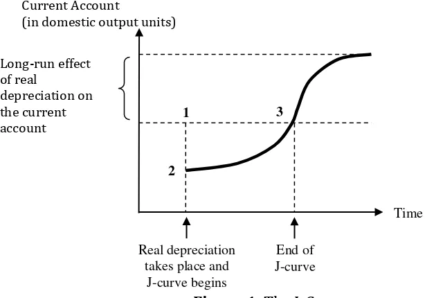
Jamilov (2010), Husman (2005), and Kapoor and Ramakrishnan (1999) explained that a change in exchange rate has two effects on trade flow, namely price effect and volume effect. The price effect means that in the short run, the depreciation will cause the price of imports more expensive and the price of exports cheaper for foreign buyers. Figure 1 shows that if the volume of imported and exported goods are not significantly change, the trade balance will gradually go down (the movement from point 1 to point 2). Since the goods and services of exports and imports are sufficiently elastic, the volume of trade will quickly response to the depreciation and the current account improves (the movement from point 2 to pont 3). Krugman and Obstfeld (2006) summarized that if there is a domination of the volume effect over the price effect, the phenomenon of Marshall-Lerner condition will be satisfied. The total effect when the plotted over time with trade balance on the y-axis will yield the J-curve.
Considering the objective of this research, the Marshall-Lerner condition can be mathematically detected by summing up the elasticity of export demand (η) and elasticity of import demand (η*). Following Krugman and Obstfeld (2006), the condition for an increase in price to improve the current account, i.e. Marshall-Lerner condition, can be formulated as follows:
η + η* > 1 (1)
194
Figure 1. The J-Curve
Source: Krugman and Obstfeld (2006)
RESEARCH METHODS Cointegration Test
As pointed out by Gujarati (2003), the existence of cointegrating relationships is indicated when two or more non stationary series have at least a linear combination which is stationary, I(0). In short, the stationary linear combination cancels out the stochastic trends in two series, proven by checking the residuals from the regressions which are stationer, I(0). Thomas (1997) noticed that the presence of cointegration for multivariate equation case is detected by applying Johansen cointegration test. The empirical result of Johansen test will be confirmed by Error Correction Model (ECM), as follows:
3
2 1 Current Account
(in domestic output units)
Long-run effect of real
depreciation on the current account
Real depreciation takes place and
J-curve begins
End of J-curve
Here, the lengths of involved for each variable is denoted as nx, np, ns, and nc. Aspointed out by Baak (2005, 2006, and 2007), the negative and significant of the estimated error correction term (ECT) coefficient ( represents the presence of long-run relationships among the variables included in the model. Since there is at least one cointegration among the variables, the causal relationship among these variables will be detected by the VECM procedures.
Data Sources
This study takes sample period from the first quarter of 1987 to the first quarter of 2011. All of calculated data were taken from Direction of Trade Statistics (DOTS) of the International Monetary Fund (IMF), International Financial Statistics (IFS) of the IMF and National Bureau of Statistics of China (NBSC).
Hypotheses Development
The dynamics of aggregate demand for exports is constructed within the basic theory of demanded exports. Specifically, as mentioned by Murianda (2008), the demanded exports (Xd) depends on price of exports goods and services (Px), real income of importing
country (Yf) and price of exports goods and services from competitor (Pc). The demanded
exports function can be constructed, as follows:
Xd = f(Px, Yf, Pc) (3)
Equation (4) shows the econometric model of how real exchange rates of RMB affects bilateral exports of Indonesia in the long run. It is constructed by referring to the equation 1 and some previous model such as Baak (2005, 2006 and 2007), Arize and Osang (2000), Widarjono (2005), and Funke and Rahn (2005). In addition, it is augmented dummy variables in order to catch up the impact of RMB devaluation in 1994.
EXijt= β0+ β 1 GDPjt+ β2 RERijt+ β3 RERVOLijt+ β4 RERCcjt+ β5 Dijt + εijt (4)
196
demanded exports. Following the work of Baak (2006), the formula for, EXijt, can be formed by simple formula as appeared in appendix.
As a proxy to measure the real income of one country, variable GDP is involved in the model, GDPjt. Data for real GPD are provided by the International Financial Statistics (IFS). It is not clear that GDP and real export has positive or negative relationship. If the estimated coefficient sign is negative, it means that demanded goods are inferior. Meanwhile, if the estimated coefficient sign is positive, it suggests that goods demanded are normal. However, when the estimated coefficient elasticity is greater than 1, it indicates that goods demanded are superior.
Real exchange rate, RERijt, represents i country currency against j’s currency. It represents the price of demanded exports. It is computed as common formula of RER in many literatures of international trade. The effect of expected coefficient of bilateral RER on the bilateral exports estimation can be significantly positive or negative. When exchange rate of exporting country depreciates and the estimated coefficient is positive, it reflects the elastic export commodity. Meanwhile, when the exchange rate of exporting country depreciates and the estimated coefficient is negative, it represents the export commodity which is inelastic. The Marshall-Lerner condition will be satisfied since the estimated coefficient of RER is greater than 1, impliying that depreciation will improve the current account and detect the existence J-curve, and vice versa. In addition, in the case of Chinese real exchange rate, RERCcjt, the measurements is also formulated in the same way by converting the subscript i into c and the interpretation of its estimated coefficient is similar with RERijt variable.
EMPIRICAL RESULTS AND ANALYSIS Unit Root Test
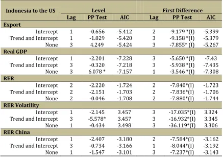
The equilibrium relationship is detected by testing the order of integration of the variables examined i.e. real exports, real GDP, RER, RER volatility, and RER China. To do so, we firstly apply the Philip-Perron (PP) test to see for both the level and the first difference. The optimal length of lag applied in the test is determined by using Aikake Information Criterion (AIC). As presented in table 1, all variables of PP statistics are lower than MacKinnon critical value, meaning that all variables are not stationary at level. However, all variables are integrated of order one I(1) indicating that they are stationary at the first difference.
Table 1: PP Unit Roots Test for the Level and the First Differences: Indonesia-US
Indonesia to the US Level
Source: IFS, DOTS and NBSC. Author’s calculation. The figures in the brackets are the order of integration
*) denotes rejection of a unit root hypothesis based on Mackinnon’s critical values at the level of
198 Cointegration Test
The optimal lags length in Johansen cointegration test are chosen based on the VAR lag order selection criteria tests, the which maximum lags length included in the tests are 1 (one) (see Appendix 1). In addition, if the I(1) variables involved are cointegrated, thus the estimated coefficient are consistent (Thomas, 1997).
Table 2. Johansen Cointegration Test
Null Test Statistic Critical Values (5%)
Hypothesis Trace Max Trace Max
r = 0 93.714 46.984* 107.346 43.420
r 1 46.730 21.361 79.341 37.164
r ≤ 2 25.368 10.954 55.246 30.815
r ≤ 3 14.414 7.568 35.010 24.252
r ≤ 4 6.846 6.387 18.398 17.148
Source: IFS, DOTS and NBSC. Author’s calculation.
*) denotes rejection of a unit root hypothesis based on Mackinnon’s critical value at at the α=1%,
5%, or 10%.
As presented in table 2, the result shows that both trace statistics and max-eigenvalue statistics confirm the presence of cointegrating vectors, implying the variables in equation (4) are cointegrated. This finding is supported by the Error Correction Model (ECM) estimation presented in table 3 showing that the estimated coefficient of Error Correction Term (ECT) in all of regression results are negative and significant at the level of significances of α= 5% and 10%. In other words, this result shows long-run relationships among variables involved.
Table 3: ECM Estimation
C GDP RER RERVOL RERC DUM ECT R2 DW 0.001 0.96* -0.07 0.002* -0.06 -0.07 -0.12* 0.27 1.87
(0.002) (0.220) (0.014) (0.001) (0.042) (0.021) (0.045)
Source: Authors’ calculation.
Notes: Standard error in parantheses
The Estimated Coefficient Interpretation
As mentioned before, this study only focuses on the impact of Chinese Renminbi on bilateral exports of Indonesia to the US in the long run, hence the short run impacts will be ignored. Equation (5) shows, the Indonesian exports are only positively influenced by GDP and bilateral real exchange rate of IDR against the US$ in the long run. The coefficient value of GDP of the US informs that offered products by Indonesian are superior product for the US people. Subsequently, 1% depreciation of IDR will turn out 0.32 percent increase in exports goods from Indonesia to the US. Since the estimated coefficient of real exchange rate is not greater than 1, the Marshall Lerner condition does not exists in the model, impliying that the depreciation of IDR might not improve the trade balance.
EXijt = 4.27 +1.52GDPjt + 0.32RERijt - 0.10RERVOLijt - 0.36RERCcjt - 0.10 Dijt (5) [3.45]* [3.77]* [ 7.32]* [ 4.37]* [ 1.57]
The asterisk (*) indicate the rejection of the null hypothesis of a zero coefficient at the 5% significance level.
Both the bilateral real volatility exchange rate of IDR against the US$, RERVOL, and bilateral real exchange rate of RMB against US$, RERC, in contrast, has negatively significant impact to the bilateral export of Indonesia to the US. It means that the exporters of Indonesia are risk averse and the relationship of exports goods between Indonesia and China in the US market is substitution, respectively. These findings are similar to Baak (2007) that also found the relationship of export goods between Korean and China in the Japan market. In contrast, Widodo and Putriani (2011) and Putriani (2010) observed that the relationship between Indonesia and China applying OLS-ECM procedures, showing complementary. The devaluation policy of RMB denoted by the dummy variables, Dijt. In
practice, it have no significant impact on the bilateral exports of Indonesia to the US.
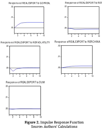
Impulse Response Function and Variance Decomposition
200
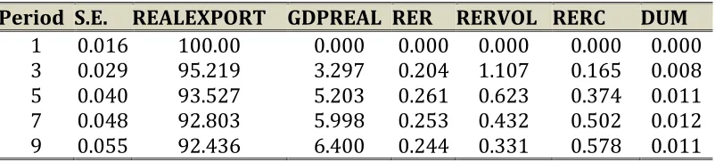
Table 4:Variance Decomposition
Period S.E. REALEXPORT GDPREAL RER RERVOL RERC DUM 1 0.016 100.00 0.000 0.000 0.000 0.000 0.000 3 0.029 95.219 3.297 0.204 1.107 0.165 0.008 5 0.040 93.527 5.203 0.261 0.623 0.374 0.011 7 0.048 92.803 5.998 0.253 0.432 0.502 0.012 9 0.055 92.436 6.400 0.244 0.331 0.578 0.011 Note: Cholesky Ordering: REALEXPORT, GDPREAL, RER,RERVOL, RERC, DUM
As pointed out by Enders (1995), the forecast error variance decomposition tells the proportion of the movements in a sequence because its own shock against other variables shock. In the other words, the variance decomposition is a calculation of variance forecast error in the percentage framed by another variable within the short run dynamics and interactions. Table 4 presents the result of variance decomposition within 1, 3, 5, 7, and 9 periods. It confirms that the real exports are mostly related to its own variation from 95.2 percent in period 3 up to 92.4 percent in period 9. The highest contributor variable on real exports changes is GDP, meanwhile, variable RER, RERVOL, RERC, and DUM shows small effects on the dynamic of real exports.
Research Analysis and Policy Recommendations
202
Second, comparing the values of estimated coefficient of RER and RERC, it implies that the depreciation of IDR will increase the exports of Indonesia to the US (0.32 percent). However, it yields smaller amount than if RMB is depreciated against the US$ (0.36 percent). In this case, the relationship between these two products is substitution, hence the depreciation of RMB will suffer Indonesian exports to the US. In the other words, the product of Indonesia is less competitive than the product from China in the US market. Therefore, this study propose to strengthen the establishment of real sectors in order to
improve the efficiency in production cost before to promote “go international”.
Third, since the Chinese government has made a conscious decision to embark on far-reaching economic liberalization and enlisted as a new member of World Trade Organization (WTO) in 2001, the exports, Foreign Direct Investment (FDI) and overall growth prospects of China have significantly increased (Rawski, 2009; Yamazawa and Imai, 2001). Data from the UN COMTRADE shows that Chinese exports have achieved a record
i.e. exceeding Japan’s exports since 2004. In 1988 the number of FTCs reached more than
5.000 with full authority in trade (Panagariya, 2006). Considering these Chinese hegemony in the Asia, in the short run the government of Indonesia should determine the variety of
exports goods so that the exports product become complementary with China’s product.
However, in the long run, the government should develop genuine products that can be competitive advantage for Indonesia.
CONCLUSIONS
This study finds that the RMB depreciation has negative impacts on the exports of the Indonesia to the US. It indicates that the relationship between Chinese and Indonesian exports to the US market is substitution. It also confirms that there no Marshall-Lerner condition indicating the J-curve phenomenon does not exist.
the efficiency cost of production, and (c) in the long run, Indonesian government should develop competitive products in international market.
Finally, this study focuses on the impact of Chinese Renminbi on the bilateral exports between Indonesia to US in the long run. The short run, equation from import side and sectoral (commodity) level analyses are excluded. For future research, it is encouraged to explore the impact of Chinese renminbi by considering from two sides (export and import) and commodity level in order to get deeper and stronger empirical analysis both in the short run and the long run.
REFERENCES
Arize, A and Osang, T. (2000). Exchange rate volatility and foreign trade: Evidence from
thirteen LDC’s. Journal of Busssines and Economic Statistics. Vol.18, No.1:10-17. Aswicahyono, H. and Pangestu, M., (2000). Indonesia’s recovery: export and regaining
competitiveness. The Developing Economies 38 (4): 454-89.
Athukorala, P. and Yamashita, N (2006). Production fragmentation and trade integration: East Asia in a global context. North American Journal of Economic and Finance, 17(3): 233-256.
Baak, S. (2005). The bilateral real exchange rates and trade between China and The U.S. Unpublished Manuscript. Department of Economics. Waseda University.
Baak, S. (2006). The Impact of The Chinese renminbi on the exports of Korea and Japan to The U.S. Unpublished Manuscript. Department of Economics. Waseda University. Baak, S. (2007). The effect of the Chinese renminbi on Korean export to Japan. The Journal of
Econometric Study of Northeast Asia. Vol. 6, No. 1: 103-112
Bloom, D, Caning, E D, Hu, L, Liu, Y, Mahal, A, and Yip, W (2006), Why has China’s economy
taken off faster than India’s. Paper presented at the 2006 PAN Asia Conference, Stanford University, http://scid.stanford.edu/events/PanAsia/Papers/Bloom.pdf . Cable, V and Ferdinand, P. (1994). China As an Economic Giant: Threat or Opportunity? Royal Institute of International Affairs 1944. Vol. 70, No. 2 (Apr., 1994), pp. 243-261
204
Fouquin, M., D. Hiratsuka and F. Kimura, (2006). Introduction: East Asia’s de facto economic integration. In Hiratsuka, Daisuke (ed.), East Asia’s De Facto Economic Integration. New York: Palgrave Macmillan. pp. 1-15.
Funke, M and Rahn, J (2004). Just how undervalued is the Chinese renminbi? World Economy, Vol. 28, No.4: 456-487
Gaulier, G., Lemoine, F., Kesenci, D.Ü., (2006).China’s specialization in East Asian production sharing, in Hiratsuka, D. (ed), East Asia’s De Facto Economic Integration. New York: Palgrave Macmillan. 135-180.
Goldstein, M and Lardy, N. (2006) .China's Exchange Rate Policy Dilemma. The American Economic Review, Vol. 96, No. 2 (May, 2006), pp. 422-426.
Gujarati, D. (2003). Basic Econometrics. Fouth Edition. New Jersey: Mc Graw Hill.
Hummels, D., Ishii, J., and Yi, K., (2001).The nature and growth of vertical specialization in world trade. Journal of International Economics, 54(1):75-96.
Husman, J. A. (2005). Pengaruh Nilai Tukar Riil Terhadap Neraca Perdagangan Bilateral Indonesia: Kondisi Marshall-Lerner dan Fenomena J-Curve. Buletin Ekonomi Moneter dan Perbankan. December 2005.
International Financial Statistics. Http:// www.elibrary-data.imf.org
Ishihara, K. (1993). China’s Conversion to a Market Economy. IDE Occasional Papers Series No. 28. Tokyo: IDE.
Jamilov, R. (2010). J-Curve Dynamics and the Marshall-Lerner Condition: Evidence from Azerbaijan. Unpublished manuscript. Available from URL: http://www.mpra.ub.uni-munchen.de/36799/
Kapoor, A. G. and Ramakrishnan, U. (1999). Is there A J-Curve? A New Estimation for Japan. International Economic Journal. Vol. 13. No.4. Winter1999.
Kwan, C. H, (2002). The rise of China and Asia’s flying-geese pattern of economic development: an empirical analysis based on US import statistics. Nomura Research Institute (NRI) Paper No. 52. [Online; cited 5 November 2006]. Available from URL:
https://www.nri.co.jp/english/opinion/papers/2002/pdf/np200252.pdf. National Bureau of Statistics of China. Http://www.stats.gov.cn/english/
Ng, F and Yeats, A., (2003). Major trade trends in East Asia: what are their implications for regional cooperation and growth? Policy Research Working Paper. The World Bank, Development Research Group Trade, June. Available from URL:
Panagariya, A, (2006). “India and China: trade and foreign investment”. Paper Presented at ‘Pan Asia 2006’ Conference, Stanford Center for International Development, http://scid.stanford.edu/events/PanAsia/Papers/Panagariya.pdf
Putriani, D. (2010). Dampak Renminbi Cina terhadap Ekspor Bilateral ASEAN5 ke Amerika Serikat. Undergraduate thesis. Faculty of Economics and Business. Universitas Gadjah Mada, Indonesia. Unpublished.
Rawski, T. (2009). China’s economy and global interactions in the long run. Discussion Paper No.53. United Kingdom: China Policy Institute of Nottingham University. Http://www.chinapolicyinstitute.org.
Srinivasan, T.N., (2006). China, India and the world economy. Working Paper No. 286, Stanford Center for International Development, July, http://scid.stanford.edu/pdf/SCID286.pdf .
Teh Jr, Robert R. (1999). The effects of a renminbi devaluation on ASEAN economies: An applied general equilibrium approach. Presented at The China-ASEAN Research Institutes Roundtable University Of Hong Kong. Hong Kong: 16-18 September 1999. Http://www.aseansec.org/2826.Htm
Widarjono, A. (2005). The impact of real exchange rate and trade balance. Jurnal Ekonomi dan Bisnis Indonesia. Vol.20. No.3: 239-249.
Widodo, T. (2008). Shifts in pattern of specialization”. Gadjah Mada International Journal of Business. January-April. Vol.10. No.1: 47-75
Widodo, T and Putriani, D. (2011). RMB Devaluation: Does It Reduce The Bilateral Exports Volume of Indonesia to the Four Selected Major Trading Countries. Paper presented at The "5th Annual Workshop, the Dynamics of Capital Flows and the Currency Competitiveness", October 12, 2011. Bulletin of Monetary Economics and Banking. The Central Bank of Indonesia
World Bank, (2006). World Development Indicators. Washington D.C.: World Bank.
World Bank, (1993). The East Asian Miracle: Economic Growth and Public Policy. Washington, D.C.: The World Bank.
206 The Formulas
Real Exports
Due to that the data of export unit value from Indonesia are incomplete, the real exports are calculated as of in the study of Baak (2006). EXijt equals to the logarithm value of the quarterly nominal imports, NIMijt, of country j from i divided by import unit value index of a country i (IMUVit) times 100.
Real Exchange Rate Volatility
The RERVOLijt represents the logarithm value of real exchange rate volatility. It is measured as natural logarithm of the absolute quarterly standard deviation of monthly real exchange rate which formulated as follows2:
RERijkrepresents the monthly real exchange rate, meanwhile is the quarterly average of monthly real exchange rates and k is the index of the months in a quarter.
2 The equation of the logarithm value of real exchange rate volatility above is a correction of
formula which has been employed by Baak (2007), as follows:
According to the equation of Baak (2007), there is a possibility to compute negative and/or zero value from standard deviation, which is impossible to be calculated. Thus, we argue that
Lag Length Criteria
Lag LogL LR FPE AIC SC HQ
0 136.2622 NA 2.09e-09 -2.960504 -2.791594 -2.892454
1 798.3695 1218.879 1.38e-15* -17.19022* -16.00785* -16.71387*
2 832.9609 58.96270* 1.44e-15 -17.15820 -14.96238 -16.27356
3 852.1160 30.03860 2.18e-15 -16.77536 -13.56609 -15.48243
4 875.9133 34.07350 3.03e-15 -16.49803 -12.27530 -14.79680
5 896.5000 26.66913 4.73e-15 -16.14773 -10.91154 -14.03820
6 913.3985 19.58690 8.43e-15 -15.71360 -9.463958 -13.19578
7 947.4973 34.87373 1.09e-14 -15.67039 -8.407292 -12.74427
8 973.1739 22.75882 1.88e-14 -15.43577 -7.159214 -12.10135
9 1008.806 26.72403 2.94e-14 -15.42741 -6.137395 -11.68470
*indicates lag order selected by the criterion
LR: sequential modified LR test statistic (each test at 5% level) FPE: Final prediction error