Sector-Specific and Spatial-Specific Multipliers in Indonesian Economy: World Input-Output Analysis

Sector-Specific and Spatial-Specific Multipliers in Indonesian

Economy: World Input-Output Analysis

M. Muchdie1), M. Nurrasyidin2)

1_{Sekolah Pascasarjana, Universitas Muhammadiyah Prof. Dr. HAMKA}

2_{Fakultas Ekonomi dan Bisnis, Universitas Muhammadiyah Prof. Dr. HAMKA}

Corresponding Author: eidmuchdie@uhamka.ac.id

Recieved: January 2018 | Revised: March 2018 | Accepted July 2018

Abstract

This article discusses on sector-specific and spatial-specific multipliers in Indonesian economy using 6-country-30 sector input-output tables for the year 2000, 2005, 2010 and 2014. The results show that firstly, in all years, there were 20 sectors with total output multipliers more than 2. Flow-on effects were higher than initial effects. These sectors should be prioritized if increasing of total output is the objective of Indonesian economic development as total output will be created with less initial efforts. Secondly, in the year of 2000, average percentage of multipliers occurred in own-sector was 56.23 per cent, and increase slightly in 2005 (57.38%) and 2010 (58.93%), but decrease in 2014 (57.98%). Correlation between total output multipliers and percentage of multipliers occurred in other-sector was positive, very strong and statistically significant. The higher total output multipliers, the higher percentage of multipliers occurred in other-sector. Thirdly, in the year of 2000, average percentage of multipliers occurred in other-countries was 21.34 per cent and decrease slightly in 2005 (20.22%) and 2010 (18.14%), but increase in 2014 (20.55%). Correlation between total output multipliers and percentage of multipliers occurred in other-countries were positive, very strong and statistically significant. The higher total output multipliers, the higher multipliers occurred in other-countries.

Keywords: total multipliers, sector-specific multipliers, spatial-specific multipliers.

JEL Classification:C67, D57

How to Cite: Muchdie, M., & Nurrasyidin, M. (2018). Sector-Specific and Spatial-Specific Multipliers in Indonesian Economy: World Input-Output Analysis. Jurnal Ekonomi Pembangunan: Kajian Ma -salah Ekonomi dan Pembangunan, 19(1), 64-79. doi:https://doi.org/10.23917/jep.v19i1.5661

DOI: https://doi.org/10.23917/jep.v19i1.5661

1. Introduction

Indonesia is the largest economy in Southeast Asia and is one of the emerging market economies of the world. This archipelago comprising five main island (Muchdie, 2011) and more than 17.000 small island (BPS, 2014), more than 250 million people lived in 34 provinces. The country is also a member of G-20 major economies and classified as a newly industrialized country (World Bank, 2017). It is the sixteenth largest economy in the world by nominal GDP and is the seventh largest in terms of GDP (PPP). Indonesia still depends on domestic market,

and government budget spending and its ownership of state-owned enterprises and the administration of prices of a range of basic goods including, rice, and electricity plays a significant role in Indonesia market economy, but since the 1990s, the majority of the economy has been controlled by private Indonesians and foreign companies (Adhi, 2015).

much the money supply increases in response to a change in the monetary base (Krugman & Wells, 2009; Mankiw, 2008). Multipliers can be calculated to analyze the effects of fiscal policy, or other exogenous changes in spending, on aggregate output. Other types of fiscal multipliers can also be calculated, like multipliers that describe the effects of changing taxes.

Literature on the calculation of Keynesian multipliers traces back to Kahn’s description of an employment multiplier for government expenditure during a period of high unemployment. At this early stage, Kahn’s calculations recognize the importance of supply constraints and possible increases in the general price level resulting from additional spending in the national economy (Ahiakpor, 2000). Hall (2009) discusses the way that behavioral assumptions about employment and spending affect econometrically estimated Keynesian multipliers.

The literature on the calculation of I-O multipliers traces back to Leontief economic IO model in 1930s to the broadening spectrum of applications over the years is well documented (Hewing & Jensen, 1987; Rose & Miernyk, 1989; Lahr, 1993; Dietzenbacher & Lahr, 2004; Bjerkholt &Kurz, 2006; Miller &Blair, 2009). The diversity of theme reflects the blossoming of input-ouput as a key analytical framework in the field of economic systems research and its sub-diciplines, with relevance to numerous reseach fields (Suh & Kagawa, 2005; Timmer and Aulin-Ahmavaara, 2007; Debresson, 2008; Wiedmann, 2009; Los & Steenge, 2010, Duarte & Yang, 2011; Tukker & Dietzenbacher, 2013; Inomata & Owen, 2014; Okuyama & Santos, 2014). In addition, input-output has established itself as an invaluable prcticl tool widely used by governments, industry and other national and international organisation (Meng et al., 2013; OECD, 2015;United Nations, 2017).

Richardson (1985) notes the growth of survey-based regional input-output models in the 1960s and 1970s that allowed for more accurate estimation of local spending, though at a large cost in terms of resources. To bridge the gap between resource intensive survey-based multipliers

and “off-the-shelf” multipliers, Beemiller (1990) describes the use of primary data to improve the accuracy of regional multipliers. The literature on the use and misuse of regional multipliers and models is extensive. Coughlin & Mandelbaum (1991) provide an accessible introduction to regional I-O multipliers. They note that key limitations of regional I-O multipliers include the accuracy of leakage measures, the emphasis on short-term effects, the absence of supply constraints, and the inability to fully capture interregional feedback effects.

chain (Hertwich & Peters, 2009; Hummels et al., 2001; Lenzen et al., 2012; Wiebe et al., 2012; Timmer et al., 2014, Los et al., 2015).

The objective of this paper is to calculates, presents and discusses on sectoral and spatial multipliers in Indonesian economy using 6-country-30sector input-output tables for the year 2000, 2005, 2010 and 2014 processed from World Input-Output Tables.

2. Method of Analysis

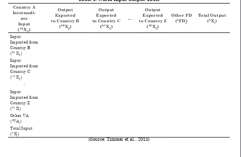
An input-output table records the “flows of products from each industrial sector considered as a producer to each of the sectors considered as consumers” (Miller & Blair, 2009). It is an “excellent descriptive device” and a powerful analytical technique (Jensen et al., 1979). In the production process, each of these industries uses products that were produced by other industries and produces outputs that will be consumed by final users (for private consumption, government consumption, investment and exports) and also by other industries, as inputs for intermediate

consumption (Oosterhaven & Stelder, 2007; Timmer et al., 2015). These transactions may be arrayed in an input-output table, as illustrated in Table 1.

The columns of Table 1 provide information on the input composition of the total supply of each product j (X_j), this is comprised by the national production and also by imported products. The value of domestic production consists of intermediate consumption of several industrial inputs i plus value added. The inter-industry transactions table is a nuclear part of this table, in the sense that it provides a detailed portrait of how the different economic activities are interrelated. Since intermediate consumption is of the total-flow type, this implies that true technological relationships are being considered. In fact, each column of the intermediate consumption table describes the total amount of each input i consumed in the production of output

j, regardless of the geographical origin of that input.

Table 1. World Input-Output Table

Country A

Figure 1.

The input-output interconnections illustrated in Table 1 can be translated analytically into accounting identities. On the supply perspective, if X_ij denote the intermediate use of product i by industry j and y_i denote the final use of product i, we may write, to each of the n products:

A_X i =

AA_X ij +

BA_X ij +

CA_X

ij + … + ZA_X

ij + AVA

i (1)

On the demand side, we know that:

A_X j =

AA_X ij +

AB_X ij +

AC_X

ij + … + AZ_X

ij + A_FD

j (2)

in which w_j stands for value added in the produc-tion of j and m_j for total imports of product j. It is

required that, for i = j, x_i = x_j, i.e., for one specific product, the total output obtained in the use or demand perspective must equal the total output achieved by the supply perspective. These two equations can be easily related to the National Accounts’ identities. In general term, equation (1) can be written as:

x = Ax + y or x = (I - A)-1_{y (3)}

National Input-Output Table of Indonesia for the year of 2000, 2005, 2010 and 2014 are available from World Input Output Data Base (Timmer et al., 2016; 2015). Calculation of total and disaggregated multipliers, sector-specific multipliers and country-specific multipliers were following West (1990) and modified formula of DiPasquale & Polenske (1980). West (1990) defined the major categories of response as: initial, first-round, industrial-support, consumption-induced, total and flow-on effects. Total effect is calculated as summation of initial, direct-effect (first-round), indirect-effect (industrial-support) and consumption induced effect (as matrix is closed to house-hold row and column, which was not calculated in this study). Flow-on effect is defined as the different between total and initial effects. Modified from DiPasquale & Polenske (1980), sector-specific multipliers of output are calculated as ∑cr_b

ij; c = 1..., n, and country-specific

multipliers of output is calculate as ∑cs_b

A,.., Z. Note that c and r are the m origin and destination countries, i and j are the n producing and purchasing sectors, cr_b

ij is the element of

inverse of Leontief matrix, m is the number of country and n is the number of sectors. Sector classifications is available in Appendices.

3. Results and Discussions 3.1. Results

3.1.1. Total Multipliers

Figure 1 presents disaggregated output multipliers in Indonesian economy for the year of 2000 and 2005. In the year 2000, 20 sectors had total output multipliers more than 2. It means that the sum of direct and indirect effects were more than the initial effects; the flow-on effects was higher than initial effect. These sectors were: Sector-5 (2.1886), Sector-6 (2.4223), Sector-7 (2.1122), Sector-8 (2.5858), Sector-9 (2.3655), Sector-11 (2.2409), Sector-12 (2.4163), Sector-13 (2.4556), Sector-14 (2.0958), Sector-15 (2.4848), Sector-16 (2.5590), Sector-17 (2.5090), Sector-18 (2.4984), Sector-19 (2.5852, Sector-20 (2.2899), Sector-21 (2.6507), Sector-22 (2.4018), Sector-24 (2.2833), Sector-25 (2.4052), and Sector-27 (2.1748). Based-on direct and indirect effects of change in final demand, these 20 sectors had more than 20 per cent of direct effects and another 20 per cent of indirect effects, made totally more than 40 per cent of total effects. It means that to increase 1 unit of total output, it only needs to increase final demand (export, for instance) by less than 50 per cent. Other 10 sectors had total multipliers less than 2; meaning that increasing 1 unit of final demand would increase total output by less than 2. Flow-on effects created were less than 1 unit.

In the year 2005, the same 20 sectors, except Sec -tor-27, had total output multipliers of more than 2. It means that the sum of direct and indirect effects were more than the initial effects; the flow-on effect was higher than initial effect. These sec-tors were: Sector-5 (2.1469), Sector-6 (2.3787), Sector-7 (2.0119), Sector-8 (2.3872), Sector-9

(2.4023), Sector-11 (2.2752), Sector-12 (2.4830), Sector-13 (2.5105), Sector-14 (2.0192), Sector-15 (2.4720), Sector-16 (2.4546), Sector-17 (2.3987), Sector-18 (2.4235), Sector-19 (2.6964), Sector-20 (2.4113), Sector-21 (2.5420), Sector-22 (2.3349), Sector-24 (2.3692), Sector-25 (2.3299), and Sec-tor-29 (2.0015). These 20 sectors had more than 20 per cent of direct effects and another 20 per cent of indirect effects, made totally more than 40 per cent of total effects. It means that to increase 1 unit of total output, it only needs to increase final demand (export, for instance) by less than 50 per cent. Other 10 sectors had total multipli -ers less than 2; meaning that increasing 1 unit of final demand would increase total output by less than 2. Flow-on effects created were less than 1 unit.

Figure-2: Disaggregated Output Multipliers in Indonesian Economy: 2010 and 2014

Source: Processed from WIOT, 2017

In the year 2014, 20 sectors that had total output multipliers were: Sector-5 (2.1556), Sector-6 (2.3709), Sector-7 (2.0760), Sector-8 (2.4843), Sector-9 (2.5824), Sector-11 (2.3540), Sector-12 (2.4180), Sector-13 (2.5223), Sector-14 (2.2594), Sector-15 (2.3170), Sector-16 (2.4013), Sector-17 (2.8648), Sector-18 (2.7206), Sector-19 (2.9370), Sector-20 (2.1205), Sector-21 (2.3658), Sector-22 (2.3470), Sector-24 (2.8499), Sector-25 (2.4035), and Sector-27 (2.0485). These 20 sectors had more than 20 per cent of direct effects and another 20 per cent of indirect effects, made totally more than 40 per cent of total effects. It means that to increase 1 unit of total output, it only needs to increase final demand (export, for instance) by less than 50 per cent. Other 10 sectors had total multipliers less than 2; meaning that increasing 1 unit of final demand would increase total output by less than 2. Flow-on effects created were less than initial effects.

3.1.2. Sector-Specific Multipliers

Sector-specific multipliers separate multipliers that occurred in own-sector and that occurred in other sectors. Table 2 presents sector-specific multipliers in Indonesian economy for the year of 2000, 2005, 2010 and 2014. In the year of 2000, on average, 56.23 per cent of multipliers occurred in own-sector. Over all, there were 17 sectors in which multipliers occurred in own-sectors were more than 50 per cent. These own-sectors were: Sector-1 (76.42%), Sector-2 (96.68%), Sector-3 (70.01%), Sector-4 (85.78%), Sector-5 (55.23%), Sector-8 (57.85%), Sector-10 (58.71%), Sector-14 (51.44%), Sector-15 (52.47%), Sector-20 (56.10%), Sector-23 (100.00%), Sector-24 (50.37%),Sector-26 (59.84%), Sector-27 (52.47%), Sector-28 (69.88%), Sector-29 (53.72%) and Sector-30 (61.39%).

it could be shown that in all sectors multipliers occurred in own-sector were higher that initial effect. It means that other effects of multipliers, for instance the direct-effect, might also be occurred in own-sector. Take for example Sector-1, multiplier occurred in own-sector was 61.29 per cent, meanwhile initial effects was 59.56 per cent. Off course, all initial effects took-place in sector. The rest of multipliers occurred in own-sector (7.27 %) might by direct effect (15.57%). In other case, multipliers occurred in own-sector might be consist of initial effect and direct effect. In Sector-2, for instance, multiplier occurred in own-sector was 96.68 per cent, meanwhile initial effect was 71.94 per cent. The rest of multiplier occurred in own-sector (24.74%) might be partly by direct effect (14.43%) and or partly by indirect effect (13.63%). Regression analysis showed that correlation between multiplier occurred in own-sector and the initial effect of multiplier was very strong (0.94) and regression coefficient was statistically significant as calculated t-statistic (14.009) was higher than critical-value of t-distribution with n-1=29 (t-table= 1.699 at α=5% or 2.045 at α= 2.5%).

In the year of 2005, average multiplier that occurred in own-sector was 57.38 per cent, a bit higher than that of 2000 (56.23%). In this year, more sectors had multipliers occurred in own-sector more than 50 per cent (21 own-sectors) compared to that in the year of 2000 (17 sectors), namely: Sector-1 (73.96%), Sector-2 (77.42%), Sector-3 (76.47%), Sector-4 (83.85%), Sector-5 (54.69%), Sector-6 (54.44%), Sector-7 (53.95%), Sector-8 (60.90%), Sector-10 (63.47%), Sector-11 (53.49%), Sector-14 (51.34%), Sector-15 (53.86%), Sector-19 (50.38%), Sector-20 (58.94%), Sector-23 (100.00%), Sector-24 (53.41%), Sector-26 (62.50%), Sector-27 (58.03%), Sector-28 (68.61%), Sector-29 (52.02%), and Sector-30 (62.73%). All initial effects occurred in own-sectors. Regression analysis shown that correlation between multiplier occurred in own-sector and the initial effect of multiplier was very strong (0.93) and regression coefficient was

statistically significant as calculated t-statistic (13.740) was higher than critical-value of t-distribution with n-1=29 (t-table= 1.699 at α=5% or 2.045 at α= 2.5%).

In the year of 2010, average percentage of total multipliers occurred in own-sector was 58.93 per cent, slightly higher than that of 2005 (57.38 %). In this year, the same number of 21 sectors had more than 50 per cent of total multipliers occurred in own-sector, namely:Sector-1 (79.28%), Sector-2 (77.82%), Sector-3 (79.29%), Sector-4 (76.42%), Sector-5 (57.76%), Sector-6 (57.77%), Sector-7 (55.46%), Sector-8 (59.04%), S-10 (55.74%), S-11 (57.03%), S-12 (51.23%), Sector-19 (56.57%), Sector-20 (63.05%), Sector-21 (50.90%), Sector-23 (100.00%), Sector-24 (65.25%), Sector-26 (63.04%), Sector-27 (59.02%), Sector-28 (68.41%), Sector-29 (56.18%), and Sector-30 (73.81%).

Table-2: Sector-Specific Multipliers in Indonesian Economy: 2000, 2005, 2010 and 2014

Year 2000 2005 2010 2014

Sector

Own-Sector

Other-Sector

Own-Sector

Other-Sector

Own-Sector

Other-Sector

Own-Sector

Other-Sector

S-1 76.42% 23.58% 73.96% 26.04% 79.28% 20.72% 78.48% 21.52%

S-2 96.68% 3.32% 77.42% 22.58% 77.82% 22.18% 77.37% 22.63%

S-3 70.01% 29.99% 76.47% 23.53% 79.29% 20.71% 79.11% 20.89%

S-4 85.78% 14.22% 83.85% 16.15% 76.42% 23.58% 76.46% 23.54%

S-5 55.23% 44.77% 54.69% 45.31% 57.76% 42.24% 56.97% 43.03%

S-6 47.54% 52.46% 54.44% 45.56% 57.77% 42.23% 55.60% 44.40%

S-7 49.53% 50.47% 53.95% 46.05% 55.46% 44.54% 53.11% 46.89%

S-8 57.85% 42.15% 60.90% 39.10% 59.04% 40.96% 56.07% 43.93%

S-9 42.66% 57.34% 41.90% 58.10% 39.42% 60.58% 38.87% 61.13%

S-10 58.71% 41.29% 63.47% 36.53% 55.74% 44.26% 55.37% 44.63%

S-11 49.76% 50.24% 53.49% 46.51% 57.03% 42.97% 56.60% 43.40%

S-12 42.61% 57.39% 42.20% 57.80% 51.23% 48.77% 50.13% 49.87%

S-13 44.15% 55.85% 42.82% 57.18% 45.48% 54.52% 43.07% 56.93%

S-14 51.44% 48.56% 51.34% 48.66% 46.36% 53.64% 45.76% 54.24%

S-15 52.47% 47.53% 53.86% 46.14% 48.18% 51.82% 47.71% 52.29%

S-16 42.74% 57.26% 43.42% 56.58% 43.59% 56.41% 42.97% 57.03%

S-17 41.25% 58.75% 46.16% 53.84% 49.98% 50.02% 49.43% 50.57%

S-18 45.58% 54.42% 46.26% 53.74% 44.54% 55.46% 43.50% 56.50%

S-19 47.11% 52.89% 50.38% 49.62% 56.57% 43.43% 55.08% 44.92%

S-20 56.10% 43.90% 58.94% 41.06% 63.05% 36.95% 61.65% 38.35%

S-21 40.96% 59.04% 46.07% 53.93% 50.90% 49.10% 47.15% 52.85%

S-22 42.74% 57.26% 44.74% 55.26% 44.02% 55.98% 43.06% 56.94%

S-23 100.00% 0.00% 100.00% 0.00% 100.00% 0.00% 100.00% 0.00%

S-24 50.37% 49.63% 53.41% 46.59% 65.25% 34.75% 64.41% 35.59%

S-25 41.91% 58.09% 43.23% 56.77% 43.15% 56.85% 42.66% 57.34%

S-26 59.84% 40.16% 62.50% 37.50% 63.04% 36.96% 62.56% 37.44%

S-27 52.47% 47.53% 58.03% 41.97% 59.02% 40.98% 57.49% 42.51%

S-28 69.88% 30.12% 68.61% 31.39% 68.41% 31.59% 68.41% 31.59%

S-29 53.72% 46.28% 52.02% 47.98% 56.18% 43.82% 56.00% 44.00%

S-30 61.39% 38.61% 62.73% 37.27% 73.81% 26.19% 74.23% 25.77%

Average 56.23% 43.77% 57.38% 42.62% 58.93% 41.07% 57.98% 42.02%

Source: Calculated from WIOT, 2017

In the year of 2014, average percentage of total multiplier occurred in own-sector was 57.98 per cent; decreasing from that at the year of 2010 (58.93%). In this year, there were 22 sectors had multiplier more than 50 per cent occurred in own-sector, namely: Sector-1 (78.48%), Sector-2 (77.37%), Sector-3 (79.11%), Sector-4 (76.46%),

Sector-30 (74.23%). All initial effects occurred in own-sectors. Direct effect of multipliers might be occurred in own-sector, indirect effect might be not. Regression analysis shown that correlation between multiplier occurred in own-sector and the initial effect of multiplier was very strong (0.87) and regression coefficient was statistically significant as calculated t-statistic (9.217) was higher than critical-value of t-distribution with n-1=29 (t-table= 1.699 at α=5% or 2.045 at α= 2.5%).

3.1.3. Spatial-Specific Multipliers

Table 3 presents spatial-specific output multipliers in Indonesian economy for the year of 2000, 2005, 2010 and 2014. In the year of 2000, all sectors had more than 50 per cent multipliers occurred in own-country. On average, percentage of multipliers occurred in own-county was 78.66 per cent; meaning that 21.34 per cent of output multipliers occurred in other countries; in Australia (0.92%), China (1.17%), Japan (2.98%), the USA (1.55%) and the rest of the World (14.72%). There were 16 sectors in which more than 20 per cent multipliers occurred in other countries, namely: Sector-6 (28.61%), Sector-8 (25.87%), Sector-9 (28.60%), Sector-11 (28.56%), Sector-12 (28.00%), Sector-13 (31.95%), Sector-14 (21.03%), Sector-15 (23.94%), Sector-16 (26.93%), Sector-17 (25.35%), Sector-18 (30.05%), Sector-19 (41.08%), Sector-20 (32.00%), Sector-21 (35.10%), Sector-25 (23.24%), and Sector-27 (23.35%).

All initial effects of multipliers occurred in own-country, but direct and indirect effects might be occurred in other countries. Analyzing import components in production would be very useful in explaining this situation. Regression analysis between multipliers occurred in own-country and initial effect of multipliers shown that correlation between them was very strong (0.85) and regression coefficients (0.53) was statistically significant as calculated t-statistic (8.547) was higher than critical-value of t-distribution with n-1=29 (t-table= 1.699 at α=5% or 2.045 at α= 2.5%).

In the year of 2005, average percentage of multipliers occurred in own-country was 79.78 per cent; 20.22 per cent occurred in other countries, in

Australia (0.90%), China (2.09%), Japan (2.37% ), the USA (0.92%) and the rest of the World (13.94%). There were 15 sectors in which more than 20 per cent of multiplier occurred in other countries, namely: Sector-6 (23.57%), Sector-8 (23.06%), Sector-9 (22.70%), Sector-11 (26.71%), Sector-12 (26.23%), Sector-13 (29.68%), Sector-15 (24.98%), Sector-16 (27.20%), Sector-17 (27.70%), Sector-18 (29.51%), Sector-19 (38.37%), Sector-20 (39.34%), Sector-21 (30.87%), Sector-24 (20.70%), and Sector-25 (22.13%).

All initial effects of multipliers occurred in own-country, but direct and indirect effects, partly or fully, might be occurred in other countries. Regression analysis between multipliers occurred in own-country and initial effect of multipliers shown that correlation between them was very strong (0.81) and regression coefficients (0.49) was statistically significant as calculated t-statistic (7.183) was higher than critical-value of t-distribution with n-1=29 (t-table= 1.699 at α=5% or 2.045 at α= 2.5%).

Table-3: Spatial-Specific Multipliers in Indonesian Economy: 2000, 2005, 2010 and 2014

Year 2000 2005 2010 2014

Country

Own-Country

Other-Country

Own-Country

Other-Country

Own-Country

Other-Country

Own-Country

Other-Country

S-1 89.79% 10.21% 87.71% 12.29% 93.50% 6.50% 91.95% 8.05%

S-2 90.53% 9.47% 92.07% 7.93% 94.01% 5.99% 93.07% 6.93%

S-3 88.19% 11.81% 92.44% 7.56% 94.63% 5.37% 93.46% 6.54%

S-4 92.28% 7.72% 89.81% 10.19% 89.01% 10.99% 87.92% 12.08%

S-5 86.07% 13.93% 86.90% 13.10% 90.59% 9.41% 88.06% 11.94%

S-6 71.39% 28.61% 76.43% 23.57% 71.40% 28.60% 65.18% 34.82%

S-7 84.88% 15.12% 86.17% 13.83% 88.46% 11.54% 85.24% 14.76%

S-8 74.13% 25.87% 76.94% 23.06% 81.37% 18.63% 77.41% 22.59%

S-9 71.40% 28.60% 77.30% 22.70% 80.92% 19.08% 76.85% 23.15%

S-10 85.75% 14.25% 84.05% 15.95% 88.37% 11.63% 86.06% 13.94%

S-11 71.44% 28.56% 73.29% 26.71% 76.66% 23.34% 71.79% 28.21%

S-12 72.00% 28.00% 73.77% 26.23% 81.30% 18.70% 77.35% 22.65%

S-13 68.05% 31.95% 70.32% 29.68% 77.36% 22.64% 71.66% 28.34%

S-14 78.97% 21.03% 81.30% 18.70% 82.28% 17.72% 79.46% 20.54%

S-15 76.06% 23.94% 75.02% 24.98% 79.42% 20.58% 76.60% 23.40%

S-16 73.07% 26.93% 72.80% 27.20% 73.90% 26.10% 71.61% 28.39%

S-17 74.65% 25.35% 72.30% 27.70% 62.04% 37.96% 60.00% 40.00%

S-18 69.95% 30.05% 70.49% 29.51% 65.13% 34.87% 62.34% 37.66%

S-19 58.92% 41.08% 61.63% 38.37% 56.74% 43.26% 53.33% 46.67%

S-20 68.00% 32.00% 60.66% 39.34% 79.55% 20.45% 76.57% 23.43%

S-21 64.90% 35.10% 69.13% 30.87% 66.57% 33.43% 71.45% 28.55%

S-22 80.80% 19.20% 81.47% 18.53% 79.70% 20.30% 75.93% 24.07%

S-23 100.00% 0.00% 100.00% 0.00% 100.00% 0.00% 100.00% 0.00%

S-24 80.93% 19.07% 79.30% 20.70% 87.40% 12.60% 84.72% 15.28%

S-25 76.76% 23.24% 77.87% 22.13% 78.95% 21.05% 75.80% 24.20%

S-26 82.94% 17.06% 87.65% 12.35% 88.61% 11.39% 86.95% 13.05%

S-27 76.65% 23.35% 81.57% 18.43% 82.99% 17.01% 80.56% 19.44%

S-28 86.36% 13.64% 86.19% 13.81% 88.95% 11.05% 88.97% 11.03%

S-29 80.06% 19.94% 83.29% 16.71% 86.33% 13.67% 84.30% 15.70%

S-30 84.77% 15.23% 85.51% 14.49% 89.69% 10.31% 89.00% 11.00%

Average 78.66% 21.34% 79.78% 20.22% 81.86% 18.14% 79.45% 20.55%

Source: Calculated from WIOT, 2017

In the year of 2014, average percentage of multipliers occurred in own-country was 79.45 per cent; 20.55 per cent occurred in other countries, in Australia (0.44%), China (4.34%), Japan (1.59%), the USA (0.85%) and the rest of the World (13.32%). There were 16 sectors in which more than 20 per cent of multiplier occurred in other countries,

effects of multipliers occurred in own-country, but direct and indirect effects, partly or fully, might be occurred in other countries. Regression analysis between multipliers occurred in own-country and initial effect of multipliers shown that correlation between them was strong (0.79) and regression coefficients (0.55) was statistically significant as calculated t-statistic (6.764) was higher than critical-value of t-distribution with n-1=29 (t-table= 1.699 at α=5% or 2.045 at α= 2.5%).

3.2. Discussions

This section discusses three important findings. Firstly, total output multipliers disaggregated into initial, direct, indirect and total effects. Flow-on effect is the different between total effect and initial effect; or flow-on effect is the summatiflow-on of direct effect and indirect effects. In all years of study, 2000, 2005, 2010 and 2014, there were 20 sectors had total multipliers of more than 2. Compared to study by Muchdie & Kusmawan (2018), Indonesian had more sectors in total output multipliers that more than 2 compared to that of the United States. There were two specific findings from total output multipliers in Indonesian economy. Firstly, all sectors with total output multipliers more than 2 had initial effects less than 50 per cent. Flow-on effects were higher than initial effects. It means that direct and indirect effects of change in final demand were higher than initial effects. These sectors should be prioritized if increasing of total output is the objective of Indonesian economic development. Total output will be created with less initial efforts. Secondly, all sectors with total output multipliers less than 2 had initial effects more than 50 per cent. Flow-on effects were less than initial effects; direct and indirect effects were less than initial effects. In other word, initial effects were higher than direct and indirect effects. If these sectors were chosen as priority sectors then more initial efforts will be needed to increase total output. This priority setting will be

inappropriate as it is not the most efficient way in producing output.

of 2005; 6.831 in the year of 2010; 7.112 in the year of 2014) were higher than critical value of t-distribution with n-1=29 (t-table = 1.699 at α =5% or 2.045 at α= 2.5%). Implication of these findings was sectors with higher total output multipliers should be prioritized in economic development if the policy settled to distribute output to other-sectors.

Thirdly, related to spatial-specific multipliers, in the year of 2005, average percentage of multipliers occurred in other-country was 21.34 per cent and decrease slightly in 2005 (20.22%) and 2010 (18.14%), but increase in 2014 (20.55%). Compared to study by Muchdie and Kusmawan (2018), in the United States economy, average percentage of multipliers occured in other-country was 11.02 per cent in the year of 2000, 12.86 per cent in the year of 2005, 13.54 per cent in the year of 2010 and 14.89 per cent in the year of 2014. Another study by Muchdie and Sumarso (2018), in Japanese economy, average percentage of multipliers occured in other-country was 9.45 per cent in the year of 2000, 11.80 per cent in the year of 2005, 13.50 per cent in the year of 2010 and 18.78 per cent in the year of 2014. There were two specific findings from spatial-specific multipliers in Indonesian economy. Firstly, almost all sectors with total output multipliers more than 2 had less than 80 per cent of total multipliers occurred in own-country; more than 20 per cent of total multipliers occurred in other-countries. Secondly, all sectors with total output multipliers less than 2 had more than 80 per cent of total multipliers occurred in own-country; less than 20 per cent occurred in other countries. This finding implies that the higher total output multipliers, the higher multipliers occurred in other-countries.

4. Conclusions

From important findings as discussed in the last the Section, some conclusions could be drawn. Firstly, total output multipliers were mostly determined by direct and indirect effects of increase in final demand. In all years, there were 20 sectors with total output multipliers more than

2 meaning that flow-on effects were higher than initial effects. Direct and indirect effects of change in final demand were higher than initial effects. These sectors should be prioritized if increasing of total output or increasing GDP is the objective of Indonesian economic development. Total output will be created with less initial efforts. Secondly, in the year of 2000, average percentage of multipliers occurred in own-sector was 56.23 per cent, and increase slightly in 2005 (57.38%) and 2010 (58.93%), but decrease in 2014 (57.98%). Correlation between total output multipliers and percentage of multipliers occurred in other-sector was positive, very strong and statistically significant. The higher total output multipliers, the higher percentage of multipliers occurred in other-sector. Thirdly, in the year of 2000, average percentage of multipliers occurred in other-countries was 21.34 per cent and decrease slightly in 2005 (20.22%) and 2010 (18.14%), but increase in 2014 (20.55%). Correlation between total output multipliers and percentage of multipliers occurred in other-countries were positive, very strong and statistically significant. The higher total output multipliers, the higher multipliers occurred in other-countries.

5. Acknowledgement

Authors thank to Director of Graduate School and Dean of Faculty of Economics and Business, Universitas Muhammadiyah Prof Dr. HAMKA (UHAMKA) for their support and encouragment. Lemlitbang (UHAMKA) for faciliting instrument to do some calculations. The comments by the anonymous referees have also been extremely useful for improving his paper.

6. References

Adhi, A. (2015). 80 Persen Industri Indonesia Disebut Dikuasai Swasta. Retrieved from http://surabaya.tribunnews. c o m / 2 0 1 5 / 0 3 / 0 3 / 8 0 p e r s e n i n d u s t r i -indonesia-disebut-dikuasai-swasta.

Cognitive Dissonance? History of Political Economy, 32 (4): 889-908.

Beemiller, R.M. (1990). Improving Accuracy by Combining Primary Data with RIMS: Comment on Bourque. International Regional Science Review, 13 (1-2): 99-101.

Bjerkholt, O. and Kurz, H.D. (2006). Introduction: The History of Input-Output Analysis, Leontief’s Path and Alternative Track. Economic Systems Reaseach, 18:331-333.

BPS (2014). Statistik Indonesia (Statistical Year Book Indonesia) 2014. Jakarta, Badan Pusat Statistk.

Coughlin, C. and Mandelbaum, T.B. (1991). A Consumer’s Guide to Regional Economic Multipliers. Federal Reserve Bank of St. Louis Review, January/February 1991:19-32.

Debresson, C. (2008). China’s Growing Pains-Recent Input-Output Reseacrh in China on China: Foreword. Economic System Research, 20: 135-138.

Dietzenbacher, E. and Lahr, M.L. (2004). Wassilly Leontief and Input-Output Economic. Cambridge: Cambridge University Press.

DiPasquale, D. and Polenske, K.R. (1980). Output, Income and Employment Input-Output Multipliers, in S. Pleeter (Ed), Economic Impact Analysis: Methodology and Applications. Studies in Applied Regional Science, Boston: Martinus Nijhoff Publishing, pp. 85-113

Duarte, R. and Yang, H. (2011). Input-Output and Water: Introduction to Special Issue. Economic System Research, 23: 341-351.

Grady, P. and Muller, R. A. (1988). On the use and misuse of input-output based impact analysis in evaluation. The Canadian Journal of Program Evaluation, 2 (3): 49-61.

Hall, R. E. (2009). By How Much Does GDP Rise if the Government Buys More Output? NBER

Working Paper 15496, National Bureau of Economic Research. Retrieved from: http:// www.nber.org/papers/w15496.pdf?new_ window=1

Harris, P. (1997). Limitations on the use of regional economic impact multipliers by practitioners: An application to the tourism industry. The Journal of Tourism Studies, 8(2): 1-12.

Hertwich, E.G. and Peters, G.P. (2009). Carbon Footprint of Nations: A Global Trade-Linked Analysis. Environmental Science and Technology, 43: 6414-6420.

Hewings, G.J.D. and Jensen, R.C. (1987). Chapter 8 Regional, Interregional and Multiregional Input-Output Analysis. Handbook of Regional and Urban Economics, 1: 295-355.

Hughes, D. W. (2003). Policy uses of economic multipliers and impact analysis, Choices Publication of the American Agricultural Economics Association, Second Quarter. Retrieved from: http://www.choicesmagazine. org/2003-2/2003-2-06.htm

Hummels, D., Ishii, J., Yi, K.M. (2001). The Nature and Growth of Vertical Specialisation in World Trade. Journal of International Economics, 54: 75-96.

Inomata, S. and Owen, A. (2014). Comparative Evaluation of MRIO Databases. Economic Systems Research, 26: 239-244.

Jensen, R.C. Mandeville, T.D. & Karunaratne, N.D. (1979). Regional Economic Planning: Generation of Regional Input-Output Analysis. Croom Helm, and London.

Krugman, P. and Wells, R. (2009). Economics. Worth Publisher, Duffield, UK.

Lahr, M.L. (1993). A Review of the Literature Supporting the Hybrid Approach to Constructing Regional Input-Output Models. Economic Systems Research, 5: 277-293.

B., Lobefaro, L. and Geschke, A. (2012). International Trade Drives Biodiversity Threaths in Developing Nations. Nature, 486:109-112.

Los, B., Timmer, M.P., and de Vries, G.J. (2015). How Global are Global Value Chains? A New Approach to Measure International Fragmentation. Journal of Regional Science, 55: 66-92.

Los, B. and Steenge A.E. (2010). Tourism Studies and Input-Output Analysis: Introduction to a Special Issue. Economic Systems Research, 22: 305-311.

Mankiw, N.G. (2008). Macroeconomics. Eight Edition, Ohio, South-Western Publishing. Meng, B., Zhang, Y. and Inomata, S. (2013).

Compilation and Applications of IDE-JETRO’s International Input-Output Tables. Economic Systems Research, 25: 122-142.

Mills, E. C. (1993). The Misuse of Regional Economic Models. Cato Journal, 13(1): 29-39.

Miller, R.E. and Blair, P.D. (2009). Input-Output Analysis – Foundations and Extensions. Cambridge, Cambridge University Press.

Muchdie, (2011). Spatial Structure of the Island Economy of Indonesia: A New Hybrid Procedure for Generation Inter-Regional Input-Output Tables.Lambert Academic Publishing, ISBN 978-3-8454-1847-6

Muchdie, M and Kusmawan, M (2018). Sector-Specific and Spatial-Sector-Specific Multipliers in the USA Economy: World Input-Output Analysis. American Journal of Economics, 8 (2): 83-92. DOI: 10.5923/j. economics.20180802.03.

Muchdie, M and Sumarso, S (2018). Sector-specific and spatial-specific multipliers in Japanese economy: World input-output analysis. International Journal of Development and Sustainability, 7 (2): 651-665.

OECD (2015). Inter-Country Input-Output (ICIO) Tables. Edition 2015, Inter-Country Input-Output (ICIO)Tables, Edition 2015

Okuyama, Y. and Santos, J.R. (2014). Disaster Impact and Input-Output Analysis. Economic Systems Research, 26: 1-2.

Oosterhaven, J. and Stelder, D. (2007). Regional and Interregional IO Analysis, Faculty of Economics and Business University of Groningen, the Netherlands, Retrieved from https://www.rug.nl/research/reg/research/ irios/download/regional-io-analysis.pdf.

Pindyck, R., and Rubinfeld, D. (2012). Macroeconomics. The Pearson Series in Economics, 8th Edition, ISBN13:978-0132857123, ISBN-10: 013285712X

Richardson, H.W. (1985). Input-Output and Economic Base Multipliers: Looking Backward and Forward. Journal of Regional Science, 25 (4): 607-661.

Rose, A. and Miernyk, W. (1989). Input-Output Analysis: The First Fifty Years. Economic Systems Research, 1: 229-272.

Siegfried, J., Allen R., Sanderson, A.R., and McHenry, P. (2006). The Economic Impact of Colleges and Universities. Working Paper No. 06-W12, Retrieved from http://www. accessecon.com/pubs/VUECON/vu06-w12. pdf.

Suh, S. and Kagawa, S. (2005). Industrial Ecology and Input-Output Economics: An Introduction. Economic Systems Research, 17: 349-364.

Timmer. M. P. and Aulin-Ahmavaara, P. (2007). New Development in Productivity Analysis within an Input-Output Framework: An Introduction. Economic Systems Research, 19: 225-227.

GGDC Research Memorandum Number 162, University of Groningen, retrieved from

http://www.ggdc.net/ publications/ memorandum/gd162.pdf.

Timmer, M.P., Dietzenbacher, E., Los, B., Stehrer, R., and de Vries, G.J. (2015). An Illustrated User Guide to the World Input–Output Database: the Case of Global Automotive Production. Review of International Economics, 23(3), 575–605. DOI:10.1111/ roie.1217.

Timmer, M.P., Erumban, A.A., Los, B., Stehrer, R., and de Vries, G.J. (2014). Slicing Up Global Value Chain. Journal of Economic Perspectives, 28: 99- 118.

Tukker, A. and Dietzenbacher, E. (2013). Global Multiregional Input-Output Frameworks: An Introduction and Outlook. Economic Systems Research, 25: 1-19.

United Nations (2017). System of Environmental-Economic Accounting 2012-Application and

Extension. New York, United Nations.

West, G.R. (1990). Regional Trade Estimation: A Hybrid Approach. International Regional Science Review, 13 (1&2), 103-118.

Wiebe, K.S., Bruckener, M., Giljum, S. and Lutz, C. (2012). Calculating Energy-Related CO2 Emissions Embodied in International Trade Using a Global Input-Output Model. Economic Systems Research, 24: 113-139.

Wiedmann, T. (2009). Editorial: Carbon Footprint and Inut-Output Analysis-An Introduction. Economic Systems Research, 21: 175-186.

7. Appendices

Appendix-1: Sector Classifications Sector

Code Descriptions

Sector-1 Crop and animal production, forestry, fishing and aquaculture

Sector-2 Forestry and logging activities

Sector-3 Fishing and aquaculture

Sector-4 Mining and quarrying

Sector-5 Manufacture of wood and of products of wood and cork, except furniture

Sector-6 Manufacture of paper and paper products

Sector-7 Printing and reproduction of recorded media

Sector-8 Manufacture of coke and refined petroleum products

Sector-9 Manufacture of chemicals and chemical products

Sector-10 Manufacture of basic pharmaceutical products and pharmaceutical preparations

Sector-11 Manufacture of rubber and plastic products

Sector-12 Manufacture of other non-metallic mineral products

Sector-13 Manufacture of basic metals

Sector-14 Manufacture of fabricated metal products, except machinery and equipment

Sector-15 Manufacture of computer, electronic and optical products

Sector-16 Manufacture of electrical equipment

Sector-17 Manufacture of machinery and equipment nor elsewhere classified,

Sector-18 Manufacture of motor vehicles, trailers and semi-trailers

Sector-19 Manufacture of other transport equipment

Sector-20 Manufacture of furniture; other manufacturing

Sector-21 Repair and installation of machinery and equipment

Sector-22 Electricity, gas, steam and air conditioning supply

Sector-23 Water collection, treatment and supply; Sewerage & waste: collection, treatment and

disposal

Sector-24 Electricity, gas and drinking water

Sector-25 Construction

Sector-26 Wholesale and retail trade and repair, accommodation and food service activities

Sector-27 Transportation, telecommunication, information and publication

Sector-28 Real estate, financial and corporate services

Sector-29 Legal & management consultancy, architectures & engineering, scientific research &

devlmnt

Sector-30 Other service activities