74
Analysis of The Impact of Inflation Reduction on Output and
Unemployment in Nigeria
Richardson Kojo Edeme*, Ugbor, I. Kalu, Chisom Emecheta, Ebikabowei Biedomo Aduku
Department of Economics, University of Nigeria, Nsukka-Nigeria *corresponding author, Email: [email protected];
Received: December 2, 2017; Accepted: January 16, 2018; Published: February 2, 2018 Permalink/DOI: http://dx.doi.org/10.17977/um002v10i12018p074
Abstract
It has been enunciated that it is possible to reduce the size of the sacrifice ratio in an economy without a corresponding increase in the rate of inflation. Besides, for the Nigerian economy, there are issues relating to the inflation-output relationship, among which is how inflation inertia impacts on inflation-output and unemployment. It is therefore apt to ascertain what Nigeria’s sacrifice ratio could be after many successful inflation reductions over the years. Adopting the Instrumental Variables Generalized Method of Moments (IV-GMM) technique and using data from1970-2015, the findings suggest that inflation inertia has a significant negative impact on the actual rate of inflation in Nigeria. It was also revealed that the percentage of a year’s real GDP that must be forgone to reduce inflation by 1 percent in Nigeria is 5.1 while 53.6 percent of output was sacrificed in 1982. Equivalently, a sacrifice of 26.6 percent of cyclical unemployment was made in the same year; while the highest percentage of GDP was sacrificed in 1990 and the lowest in 2007.
Keywords: Inflation inertia, sacrifice ratio, output, unemployment JEL Classification: C22, E61, P44
INTRODUCTION
75
There is a common notion that the size of the sacrifice ratio depends on how inflation rate is reduced. Thus inflation reduction and the output cost of disinflation have generated two groups of economists. The first group have focused on the speed of disinflation. This group is further divided into the rapid (or cold-turkey) disinflation and the moderate disinflation views. The cold-turkey view suggests that monetary authority should adopt a rapid or a "cold turkey" approach to inflation reduction. The supporters of the cold turkey approach believed that gradualism raises the probability of future reversals and may have no favorable impact on inflationary expectations. On this basis, the cold turkey approach is less costly because inflation expectations adjust sharply and therefore preferable. The supporters of gradualism, on the other hand, pointed out that wages and prices, which exhibit persistence behavior, can adjust smoothly to tighter monetary policy, thus moderate disinflation is preferable (Kinful, 2007).
The second group however focussed on identifying the sources of inflation persistence and analyzing the implications of inflation inertia, capital mobility, and trade openness for the pursuit of cost-reducing strategies. Trade openness also has two views. The first explained that in an open economy inflationary policies depreciate the real exchange rate. And real exchange rate depreciation will increase the inflation rate at any given output level. This effect is stronger when the economy is more open. As a result, trade openness reduces the sacrifice ratio. The second view, on the other hand, posits that trade openness makes demand for domestic output less dependent on domestic income. This makes the firms’ optimal prices less responsive to changes in domestic output. This means that trade openness increases the sacrifice ratio (Daniels & VanHoose, 2007). But with respect to capital mobility, it is the view of Celasun (2005) that disinflation is likely to entail larger output losses in countries with more open capital accounts. This suggests that the higher expected costs of disinflation in the context of higher capital mobility could temper policymakers’ incentives to create an inflationary scenario.
76
policy. It also indicates the credibility of monetary policy by the central bank (Lendvai, 2004; Fuhrer, 2009).
Countries reduce inflation by using tight monetary and fiscal policies to slow the growth rate of aggregate demand. In Nigeria, the monetary authority, through the CBN has over the years adopted tight monetary policy to reduce the inflation rate. Periods in which the monetary policy was tightened include 2008, 2010 and 2012. In 2008, the Monetary Policy Rate (MPR) was reviewed twice in the second quarter, owing to inflationary pressure. The tight monetary policy was coupled with the global credit crunch in late 2008. In 2010, the CBN adopted tight monetary policy. The Monetary Policy Rate was reviewed upwards six times during the year, in line with the liquidity conditions. Interest rates were generally higher than in the preceding year. Another tight monetary policy stance was maintained in 2012. Growth in money supply was modest, reflecting the tight monetary policy stance. Money supply (M2) was below the indicative growth benchmark of 24.6 %
to 15.4 % (CBN 2015; 2014; 2013 and 2012). The achievement of price stability is the core mandate of monetary policy of central banks across the globe. To this end, central banks, in recent times, have leaned towards employing multiple measures, including the effective conduct of monetary policy. To reduce inflation, tight monetary and fiscal policies must be used. However, at the same time, a policy of low inflation is costly for the economy concerned. Inflation reductions result in short-term costs associated with losses in output (Evans & Nicolae, 2012; Dramani & Thiam, 2012).
77
LITERATURE REVIEW
The origin of the trade-off between inflation and unemployment began with the seminar work of Phillips (1958). On this, Abel, Bernanke, & Croushore (2008) used unemployment and nominal wage growth from Britain over 97 years and found that, historically, unemployment tended to be low in years when nominal wages grew rapidly and high in years when nominal wages grew slowly. This was however shifted slightly by focusing on the link between unemployment and inflation. During the late 1950s and the 1960s, a negative relationship between unemployment and inflation was established. During the 1960s some economists argued that, by accepting a modest amount of inflation, macroeconomic policymakers could keep the unemployment rate low indefinitely. This belief originated during the 1960s when rising inflation was accompanied by falling unemployment. These trade-offs arise because of the existence of irreconcilable conflicts among policy objectives. However, in the early 1970s, the relationship between inflation and unemployment failed to hold. This led to the birth of the inflation-expectation augmented Phillips Curve (Gordon, 1972; Akerlof, Dickens & Perry, 2000; Abel, Bernanke, & Croushore, 2008; Humphrey, 1985).
It has however been argued that when the public correctly predicts aggregate demand growth and inflation, unanticipated inflation is zero, actual unemployment equals the natural rate, and cyclical unemployment is zero. However, if aggregate demand growth unexpectedly speeds up, the economy faces a period of positive unanticipated inflation and negative cyclical unemployment. Similarly, an unexpected slowdown in aggregate demand growth could occur, causing aggregate demand to rise more slowly than expected; for a time unanticipated inflation would be negative (actual inflation less than expected) and cyclical unemployment would be positive (actual unemployment greater than the natural rate). The relationship between unanticipated inflation and cyclical unemployment can be shown as follows:
� − �� = −ℎ �–ū . . . (1)
where� − �� = unanticipated inflation (the difference between actual inflation � and expected inflation, ��), �–ū = cyclical unemployment (the difference between the actual unemployment rate, �, and the natural unemployment rate, ū), h = a positive number that measures the slope of the relationship between unanticipated inflation and cyclical unemployment. The mathematical expression of the idea that unanticipated inflation will be positive when cyclical unemployment is negative, negative when cyclical unemployment is positive, and zero when cyclical unemployment is zero is shown in the equation below:
� = �� − ℎ �–ū . . . (2)
78
Based on historical disinflationary episodes experienced by some countries. Cecchetti & Rich (2001); Belke & Böing (2014) separately applied structural vector autoregressive technique and found that most countries had sacrifice ratios of between –1 and 2 percent of real GDP for a reduction in inflation of one percentage point. Dholakia (2014) estimated the sacrifice ratio and cost of inflation for the Indian economy. Interestingly, the sacrifice ratio turns out to be in a narrow range of 1.8 to 2.1 for deliberate deflation and 2.8 for inflation. The benefits of one percent reduction in inflationary trend were at best 0.5 percentage increase in long-term growth of output that occurs after 4-5 years. This outcome was at variant with Liao & Hu (2013) who examined the influencing factors of inflation persistence in China’s economy using the DSGE approach. The authors found that inflation persistence mainly came from the persistence of the money supply, while money supply uncertainty, the reaction coefficient of monetary growth to productivity, productivity persistence and productivity uncertainty had a smaller impact on inflation persistence. Similarly, Leitemo & Røste (2005) estimated the sacrifice ratio in six small open economies, through the simulation of estimated VAR models where the historical monetary policy has been identified. They estimated the sacrifice ratio before and after the introduction of explicit inflation targeting and found that the sacrifice ratios declined after the introduction of inflation targeting variables.
The study by Dramani & Thiam (2012) calculated the sacrifice ratio in West African Economic and Monetary Union (WAEMU) zone and the findings shows that sustained decline of 1% inflation rate inherent in a monetary shock leads to a cumulative decline of 1.3% growth rate in Senegal, and 0.06% in Benin. Another contribution to the literature is Evans & Nicolae (2012) who focused on the relative impact of the main drivers of the sacrifice ratio: initial inflation, the speed of disinflation and imperfect credibility. Their findings revealed that 75% of the sacrifice ratio was attributable to the initial inflation rate, 14% to the initial lack of credibility and 11% to the speed of disinflation. Their conclusion was that for the range of inflation rates considered, what matters most for the sacrifice ratio was the scale of the disinflation, followed by the degree of credibility and the speed of disinflation.
79
(2000) estimated the sacrifice ratio for the EMU countries for the period 1960-1998 and examine whether there was enough cross-country similarity in the relationship between inflation and unemployment to assume that a common sacrifice ratio existed for these countries. From the results, it was found that there was no evidence of long-run, but short-run trade-off between inflation and unemployment. The study also revealed that the values of the estimated sacrifice ratios of the EMU countries range from 0.48% in the case of Portugal to 2.02% in the case of Finland. They came to the conclusion that all the EMU countries do not have a common sacrifice ratio.
Coffinet, Matheron, & Poilly (2007) adopted an ad hoc method, a structural VAR approach, and a general equilibrium models, covering 1985Q1- 2004Q4 to estimate the sacrifice ratio for the euro area and find the sacrifice ratio to be between 1.2 and 1.4%. Implied is that the short-term cost of a 1 percent permanent decline in inflation was over 1 GDP point. It was further pointed out that the impact of a decline in nominal wage stickiness is limited, and greater wage stickiness leads to a rise in the sacrifice ratio. In addition, the impact of a change in wage stickiness is asymmetrical, as an increase in stickiness has a particularly negative effect on the sacrifice ratio. Similarly, Kinful (2007) applied three methods to estimate the size of the sacrifice ratio for Ghana. The estimated sacrifice ratios indicates that a permanent 1 percent drop in inflation results in an output lose within the range of 0.001 to 5.1 percent. From this finding, it can be argued that if a disinflation process persists and policies are consistent and credible, the economy may eventually adjust to the new monetary policy regime and output and employment losses may only be transitory.
Daniels & VanHoose (2006) studied the linkage between openness, the sacrifice ratio, and inflation and conclude that greater openness raises the sacrifice ratio but dampens the inflation bias. It was argued further that failure to observe an inverse relationship between openness and the sacrifice ratio did not necessarily imply that the time-inconsistency approach adopted is irrelevant to understanding the openness inflation relationship. The study by Formánek & Hušek (2005) provided two estimates of sacrifice ratio for the Czech economy and found that there was a good probability that the sacrifice ratio was negative during the transition period analyzed, with relatively low absolute value. In support of this, Roberts (2007) contend that in order to improve sustainable growth of an economy, the impact of a reduction in inflationary trend must be considered as a potential policy for stimulating the growth process.
80
METHOD
The sacrifice ratio is based on the theoretical argument that given the potential output level; any attempt to reduce inflation requires a reduction in current period output. This study shall adopt the expectations-augmented Philips curve theory. The expectations-augmented Phillips curve was developed by Friedman and Phelps in 1970. The theory explained the relationship between unanticipated inflation and output gap (demand pressure). The expectations-augmented Phillips curve theory explained that the relationship illustrated by the original Phillips curve depends on the expected rate of inflation and potential output. The theory starts by defining unanticipated inflation �∗ = ��− �� as a function of output gap ��– ��∗ such that:
��− �� = − ��– ��∗ . . . (3) where:
��∗ = ��− �� = unanticipated rate of inflation
�� = actual rate of inflation
�� = inflation expectation
�� = actual output
��∗ = potential output; and
= slope of unanticipated inflation due to a changes in output gap.
For the fact that the slope coefficient is negative, measures the rate of decline in inflation due to a percentage reduction in actual output. The expectation augmented Philip’s curve is based on the adaptive expectation hypothesis so that the expected inflation is adapted from previous rate of inflation. Hence �� = ∅��− and substituting into (3) yields:
��− ∅��− = − ��– ��∗ . . . (4) Adding ∅��− to both sides of (4) yields the following:
�� = ∅��− − ��– ��∗ . . . (5)
Equation (5) is the aggregate supply function which specifically shows that actual inflation depends on past inflation (or inflation inertia) and the output gap. However, (5) does not explicitly define the output loss associated with a percentage decline in inflation. This can be derived by defining output gap in terms of inflation. Thus rearranging (5) yields the following:
− ��− ��∗ = ��− ∅��− . . . Dividing both sides of (6) by − and factorising yields the following:
��− ��∗ = − − ∅ �� . . .
Equation (7) shows that output gap depends on the rate of inflation.
As argued by Çetinkaya & Yavuz, (2002); Kinful (2007); Abel, Bernanke, &
81
percentage reduction in inflation. In line with this, the sacrifice ratio can be estimated as:
= − ∅ . . .
Estimating the sacrifice ratio involves first, the estimation of equation (7) and the sacrifice ratio is then computed as 1 less the coefficient on expected inflation divided by the coefficient of the output gap.
Model Specification
Following the predictions of the expectation-augmented Philip’s curve, the relevant functional form for this study can be expressed as:
� �� = � ��− , � � . . . where:
Inflt = actual rate of inflation at time, t
Inflt-1 = expected rate of inflation at time, t
opgap = output gap, measured as the difference between real output (real GDP) and potential output.
The model for estimation following the expectation-augmented Philip’s curve approach is then specified as:
� �� = + � ��− + � �+ �� .
where: δ = coefficient of output gap, = coefficient of inflation inertia, ut =
Stochastic error term and other variables remain as previously defined
After estimating (10) the Output Cost of Inflation reduction (OCI) will then be estimated as
��� = − . . .
The larger the impact of demand pressures on inflation, the lesser the output loss due to a percentage reduction in inflation, and vice versa. In the same vein, the larger the magnitude of inflation inertia the lower the output loss due to a percentage reduction in inflation, and vice versa. Since time series are characterized as random walks the following first differenced form of equation (10) shall be estimated and the output cost of inflation will be estimated accordingly:
∆� �� = � + � ∆� ��− + � ∆ � �+ � .
Estimation Technique
This study adopts the Instrumental Variables Generalized Method of Moments (IV-GMM) estimation technique. It is more appropriate for the fact that the OLS technique assumed that the explanatory variables in a regression model are not correlated with the error term if this assumption does not hold then the standard errors and by implication, the usual t-statistics, F-statistic and other traditional statistics for hypothesis testing will be invalid. Since the lagged dependent variable (inflt-1) enters equation (10) and (11) as an explanatory variable not only is it
82
variable. If the explanatory variable significantly explains changes in the dependent variable, apart from the endogeneity bias, this will also lead to collinearity, which will invalidate the usual test statistics.
Our estimation begins with the estimation of potential output. This necessitates filtering the real GDP data. The essence of this is to obtain the potential output, which shall be used to compute the output gap. A widely used technique in the literature to filter a time series is the Hodrick–Prescott filter (herein referred to H-P filter onwards). The primary objective of this approach is to estimate a stationary cyclical component that is driven by stochastic cycles within a specified range of periods.The trend component τt is calculated by the difference τt= yt − ct.
where: τt is the trend component and ctis the cyclical component while yt is a
time-series.
In the view of Razzak (1997), the technique specifies a trend in adata and can be filtered by removing the trend. The smoothness of the trend depends on a smoothing parameter, λ. The trend becomes smoother as λ → ∞. This technique has withstood the test of time and can be applied to non-stationary time series (series containing one or more unit roots in their autoregressive representation). They recommended setting λ to 1,600 for quarterly data. However, there are rescaled values worked out by Ravn and Uhlig (2002). The study, therefore, adopts the H-P filter technique to estimate the potential output; using Ravn and Uhlig (2002) rescaled default value of 6.25 for λ.
Data for the study are from different sources. Inflation and real gross domestic product were sourced from Central Bank of Nigeria (CBN) Statistical Bulletins. Output gap is obtained by first generating the potential output using H-P Filter Technique and secondly subtracting it from real gross domestic product. STATA 12 was used for empirical estimation.
RESULT AND DISCUSSION Test for unit root
The Augmented Dickey-Fuller unit root test approach is adopted to test for the stationarity, and the Engle-Granger technique is used to test for cointegration. The unit root test results are presented in table 1. The results show that the series are non-stationary at level, except the output gap which is stationary at five percent in its level form.
Table 1. Augmented Dickey-Fuller Unit Root Test Results
Variable ADF – Statistic Model Lag
Note * denotes significance at 5% and the rejection of the null hypothesis of presence
of unit root. The optimal lag lengths were chosen according to Akaike’s Final
83
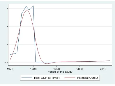
Figure 1. Real Output (RGDP) and Potential Output (PO) Source: Author’s Plot (2017)
In figure 1, the output gap in Nigeria during the period of study display both positive and negative estimates, indicating that Nigeria’s economy over the years operates significantly above and below its potential level. In other words, there were periods the economy operates above potential level and periods it operates below potential level. The Hodrick-Prescott filter estimates shows that during 1970 and 1971Nigeria’s economy operates significantly above its potential level. Periods the economy out-performed its potential level include 195-1980, 1985-1991, 2003-2006, and 2010-2013. On the other hand, periods the economy performed below its potential level are 1972-1974, 1981-1984, 1992-1997, 1999-2002 and 2007-2010. The highest positive estimate was recorded in 1980 while the lowest positive estimate was in the year 2012, to the tune of 11906.22 and 0.8290405 respectively. Similarly, the highest and lowest negative estimates were respectively -12198.68 and -.2918091 in 1981 and 2007.
Table 2. Estimation results Independent
Variables
Coefficients Standard Errors Z P-value
INFt-1 -0.199735 0.0748071 -2.67 0.000
OPGAP 0.2364701 0.1014893 2.33 0.002
Constant 0.395713.4 0.1998552 1.98 0.030
R2 0.6837 Wald chi2(5) 20.85
Prob > chi2 0.0000 Source: Author’s Computation (2017)
0
1970 1980 1990 2000 2010
Period of the Study
84
The estimated result is presented in table 2. The result revealed that a percentage increase in inflation inertia reduces the actual rate of inflation by 0.2 percent. Also, past levels of inflation have an influence on the current level of inflation. This also means that inflation in Nigeria response significantly to inflation shocks. On the other hand, an increase in the output gap leads to 0.24 percent increase in the actual rate of inflation. This means the more the output gap, is the more the inflation rate. It also means that when the economy performs below potential level by a unit in terms of output, actual inflation as well increases by 24 percent. This could be due to the under developed nature of the production processes which leads to the actual output below potential level and thus high inflation rates as commonly found in developing economies. The significant probability value of 0.002 indicates that the output gap in Nigeria has a significant impact on the rate of inflation. To estimate the output cost of inflation reduction in Nigeria, the estimated coefficients of inflation inertia and the output gap are
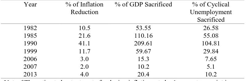
The above shows an estimated sacrifice ratio coefficient of 5.1. This means that the percentage of a year’s real GDP that must be forgone to reduce inflation by 1 percent in Nigeria is 5.1. In order words, for every percentage point, that inflation is to fall in Nigeria, 5.1 percent of one year’s GDP must be sacrificed. Based on this result and following Okun’s law which says that a change of 1 percentage point in the unemployment rate translates into a change of 2 percentage points in GDP, we go a step further to estimate the percentage sacrifice of Nigeria’s GDP at years when inflation rate is reduced from 2 digit to single digit and the corresponding cyclical unemployment that is sacrificed. The result is presented in table 3 below:
Table 3. Inflation rate reduction and percentages of GDP and cyclical unemployment Note: *The estimated output cost of reducing inflation rate by 1 percentage point is 5.1, which is used to compute the percentages of GDP and cyclical unemployment sacrificed.
85
In 1982, the inflation rate was reduced by 10.5 percent. The reduction in inflation rate results to 53.55 percent of the 1982 GDP sacrificed in the short run. Equivalently, this reduction in inflation led to a sacrifice of 26.58 percentage points of cyclical unemployment in the same year. This is similar to other years as shown in the table. The highest percentage of GDP was sacrificed in 1990 with 41.1 percent inflation rate reduction. Also, the highest cyclical unemployment was sacrificed in the same year. The year marked a very low and stable inflation rate after the drastic inflation rate reduction. On the other hand, the lowest percentage of GDP (10.2%) was sacrificed in 2007 with 2 percentage point reduction of the inflation rate, while the cyclical unemployment rate is 5.1 percent. Furthermore, years of rapid disinflation rate recorded higher percentage of GDP sacrificed, as well as higher sacrifice of cyclical unemployment as in the case of 1985 and 1990; whereas, years of moderate disinflation rate is associated with lower sacrifice of the percentage of GDP as recorded in 2007. This finding is in line with the views of the cold-turkey and the gradualist approaches to disinflation. With respect to the former, disinflation is done rapidly but with higher sacrifice ratio while for the later disinflation is carried out gradually with low output cost. Therefore the different sacrifice ratios of 1990 and 2007 for instance, are as a result of different speed of disinflation.
CONCLUSION
Using the Instrumental Variables Generalized Method of Moments (IV-GMM) regression technique, this study has demonstrated that inflation inertia has a significant negative impact on the actual rate of inflation in Nigeria. Any change in the expected rate of inflation leads to an inverse change in actual rate of inflation. Also, the output cost of inflation reduction in Nigeria was estimated as 5.1. Implied is that the percentage of a year’s real GDP that must be forgone to reduce inflation by 1 percent in Nigeria is 5.1. The reduction in inflation rate results to 53.55 percent of the 1982 GDP sacrificed in the short run. Equivalently, this reduction in inflation led to a sacrifice of 26.58 percent of cyclical unemployment in the same year. The highest percentage of GDP was sacrificed in 1990 with 41.1 percent inflation rate reduction. Also, the highest cyclical unemployment was sacrificed in the same year, while the lowest percentage of GDP (10.2%) was sacrificed in 2007 with 2 percentage point reduction of the inflation rate. From the findings, it is imperative that any plan to reduce inflation rate and the rate of reduction should be publicly announced early. This will reduce personal expectations formed by workers and firms that determine the wages and prices, and therefore there will be a common expectation of inflation. This will be more effective in reducing inflation rate even without higher output cost of the disinflation. Policymakers should put the creditability of inflation reduction policy a priority. In this way, disinflation can be achieved without any significant reduction in output.
REFERENCES
Abel, A.B., Bernanke, B.S., & Croushore, D. (2008), Macroeconomics, 6th Edition, Boston, United States, Pearson Education, Inc
86
Bakare, S. A. (2011). The trade-off between inflation and economic growth in Nigeria: The Phillips relation approach. China-USA Business Review, 10(10): 928-935.
Belke & Böing (2014). Sacrifice Ratios for Euro Area Countries-New Evidence on the Costs of Price Stability. Ruhr Economic Papers No. 520. Available from: http://dx.doi.org/10.4419/86788595
Brito, R. D. (2010). Inflation targeting does not matter: another look at OECD economies’ output sacrifice ratios. Insper Working Paper WPE: 215/2010. Central Bank of Nigeria (CBN, 2015). Statistical Bulletin, Abuja, December Central Bank of Nigeria (CBN, 2014). Annual Report and Statement of Account,
Abuja.
Central Bank of Nigeria (CBN, 2013). Annual Report and Statement of Account, Abuja.
Central Bank of Nigeria (CBN, 2012). Annual Report and Statement of Account. Abuja.
Central Bank of Nigeria (CBN, 2011). Annual Report and Statement of Account, Abuja.
Central Bank of Nigeria (CBN, 2010). Statistical Bulletin, Abuja. Central Bank of Nigeria (CBN, 2009). Statistical Bulletin, Abuja.
Cecchetti, S. G. &Rich, R. W. (2001). Structural estimates of the U.S. sacrifice ratio, Journal of Business & Economic Statistics, 19(4), 416-427.
Celasun, Y. (2005). Inflation and disinflation. Research Bulletin, 6(1), 1-12
Çetinkaya, A. A., & Yavuz, D. (2002). Calculation of output-inflation sacrifice ratio: The Case of Turkey. Central Bank of the Republic of Turkey Research Department Working Paper No 11.
Coffinet, J., Matheron, J., & Poilly, C. (2007). A structural evaluation of the sacrifice ratio in the euro area. Banque de France Digest, No. 60, April. Coffinet, J., Matheron, J., & Poilly, C. (2007), Estimating the sacrifice ratio for the
euro area. Banque de France Bulletin Digest, 160, 1-14
Cuñado, J. & de Gracia, F. P. (2000). Sacrifice ratios in the emu countries: An empirical analysis. Available at: http://www.fedea.es/hojas/publicado.html Daniels, J. P. &VanHoose, D. D. (2007). Trade Openness, Capital Mobility, and
the Sacrifice Ratio. Department of Economics Working Paper No. 03, Marquette University. Retrieved from http://epublications.marquette.edu/ econ workingpapers/41
Daniels, J. P &VanHoose, D. D. (2006). Openness, the sacrifice ratio, and inflation: Is there a puzzle?” Journal of International Money & Finance, 25: 1336-1347.
Dholakia, R. H. (2014). Sacrifice ratio and cost of inflation for the Indian economy. Indian Institute of Management Working Paper No. 02-04.
Direkçi, T. B. (2011). Determination of the sacrifice rate in Turkey, Brazil, and Italy: A comparison among countries. Journal of Development & Agricultural Economics, 3(7): 335-342
Dramani, L. &Thiam, I. (2012). Sacrifice Ratio in West African Economic and Monetary Union (WAEMU). Journal of Contemporary Management, 61-70.
87
Formánek, R. & Hušek, T. (2005). Estimation of the Czech Republic sacrifice ratio for the transition period. Prague Economic Papers, January
Fuhrer, F. (2009). Inflation persistence. Federal Reserve Bank of Boston Working Paper No. 09-14. Available at: http://www.bos.frb.org/economic/wp/ index.htm.
Gordon, R. J. (1972). Wage-Price controls and the shifting Phillips curve, Brookings Papers on Economic Activity, 1972 (2): 385, https://doi.org/10.2307/2534182.
Humphrey, T. M. (1985). The evolution and policy implications of Phillips curve analysis. Federal Reserve Bank of Richmond Economic Review, 3-22. Kinful, E. (2007). Estimation of short run trade-offs between stability and output,
Bank of Ghana Working Paper RD.
Leitemo, K. & Røste, O. B. (2005). Measuring the sacrifice ratio: Some international evidence.
Lendvai, J. (2004). Inflation inertia and monetary policy shocks. Institute of Economics Hungarian Academy of Sciences Discussion Papers No. 17 Liao, Y. & Hu, R. (2013). Who influenced inflation persistence in China? A
comparative analysis of the standard CIA model and CIA model with endogenous money, SAJEMS Special Issue, 16, 16-27.
Mazumder, S. (2014). Determinants of the sacrifice ratio: Evidence from OECD and non-OECD countries, Economic Modelling, 40: 117-135, https://doi.org/10.1016/j.econmod.2014.03.023.
Migap, J. P. (2011). Is monetary policy the best instrument for inflation targeting in the Nigerian economy? Journal of Business & Organizational Development, 3, 35-43.
Moriyama, K. (2011). Inflation inertia in Egypt and its policy implications, International Monetary Fund Working Paper No. 160.
Muñoz-Torres, R. I. (2005). Inflation targeting in emerging economies: A comparative sacrifice ratio analysis, Dynamic Models and Their
Applications in Emerging Markets, 77-108,
https://doi.org/10.1057/9780230599598_6
Razzak, W. (1997). The Hodrick-Prescott technique: A smoother versus a filter, Economics Letters, 57(2), 163-168, https://doi.org/10.1016/s0165-1765(97)00178-x.
Roberts, J. M. (2007). Learning, sticky inflation and the sacrifice ratio. Kiel Working Paper No. 1365. Available from: http://www.ifw-kiel.de/pub/kap/kapcoll/kapcoll_02.htm.
Serju, P. (2009). Estimating the output cost of disinflation: an application to Jamaica and Trinidad & Tobago, Business, Finance & Economics in Emerging Economies, 4(1), 118-148.