Electricity subsidies for agriculture: Evaluating the impact
and persistence of these subsidies in India
DRAFT
Reena Badiani
∗Katrina K. Jessoe
†‡March 31, 2011
Abstract
In India, expenditure on electricity subsidies for agriculture, an input subsidy aimed at improving agricultural productivity and the incomes of the agricultural work force, exceeds that spent on health or education. Yet the benefits and beneficiaries of these policies have been unexplored. This paper develops and empirically tests a model that describes the chan-nels through which these subsidies should impact agricultural productivity. To isolate the impact of electricity prices on groundwater extraction and agricultural revenues, we exploit year-to-year variation in state electricity prices across districts that differ in hydrogeological characteristics. We find that a 10 percent decrease in subsidies would reduce groundwater extraction by 4.3 percent, costing farmers 13 percent in agricultural revenues. As predicted, electricity subsidies increased agricultural productivity along both the intensive - crop yields - and extensive - crop acreage - margins. We calculate small inefficiency costs from these subsidies; roughly 96 to 97 paise of every Rupee spent by the government is passed along to consumers and producers.
∗World Bank
†Dept. of Agricultural and Resource Economics, UC Davis
‡Corresponding author e-mail: [email protected]; phone:(530)-752-6977
1
Introduction
Governments in developed and developing countries have pursued a variety of poverty alleviation programs including income transfers, price supports for crops (Lichtenberg and Zilberman 1986), subsidies for agricultural inputs (Gulati 1989), health policies such as nutritional supplements and vaccination programs, and educational subsidies. A large literature has evaluated the impact of conditional cash transfer programs (De Janvry and Sadoulet 2006 , Schultz 2004), health programs (Miguel and Kremer 2004) and educational programs (Kremer 2003) on education, health and income in developing countries, finding that these programs achieve distributional gains at the expense of efficiency. In this broad literature, the effect of one dominant poverty alleviation program - electricity subsidies for agriculture - has been overlooked. Nowhere is the program more pronounced than in India, where the amount spent on electricity subsidies for agricultural users exceeds state spending on health or education (Birner et al. 2007).
In India, electricity subsidies enabled agricultural users to access electricity at prices below the marginal cost of supply, thereby lowering the cost of irrigation and groundwater extraction, an essential input in agricultural production. These electricity subsidies may also generate economic inefficiencies. They may distort decisions over electricity consumption and groundwater extraction and induce individuals to grow more water intensive crops. Given the size of electricity subsidies for agriculture in India as well as in other developing countries, the economic consequences of this poverty alleviation strategy may be large. In this paper, we analyze the impact of electricity subsi-dies for agriculture on electricity consumption, groundwater extraction, agricultural productivity and crop choice in India. We then consider the beneficiaries of these subsidies, namely the demo-graphics of the agricultural users that benefit from this policy. Lastly, we quantify the deadweight loss generated by this policy to evaluate the effectiveness of agricultural electricity subsidies as a government transfer.
The effect of these subsidies on the electricity sector has been widely discussed, with many attributing the poor and unreliable electricity service in India to these subsidies. In 2000, agricul-tural users in India consumed 32.5% of electricity but contributed only 3.36% of revenues. The lack of revenue generated from agricultural consumers has caused State Electricity Boards (SEBs) to operate at an annual loss. In 2001, the SEBs’ rate of return on capital amounted to -39.5% (Tongia, 2003). This negative profit is largely fueled by increased expenditure on agricultural electricity subsidies and a decline in the cross-subsidies provided by the commercial and industrial sectors.1
Anecdotal evidence suggests that these subsidies are not without their benefits. The expansion and uptake of tube wells for irrigation was largely expedited by subsidized electricity prices, which
1
reduced the price of groundwater extraction. In turn, this growth in irrigation increased agricul-tural yields, lowered food prices, increased demand for agriculagricul-tural labor and disproportionately benefited landless farmers (Briscoe and Malik 2006, Modi 2005). However, these benefits may have come at the cost of groundwater exploitation (Strand 2010). India has increasingly relied on groundwater extraction for agriculture and is currently the largest extractor of groundwater, consuming 250 cubic km of groundwater annually. As demand for groundwater increases, extrac-tion in some districts has begun to exceed the replenishable supply. Between 2002 and 2004, the percentage of districts reporting exploited groundwater resources increased from 8% to 17%.2
Our theoretical model builds on existing models of groundwater extraction and agricultural production (Provencher and Burt 1989). We assume an electricity subsidy will increase electricity consumption, and then predict that the subsidy will increase demand for groundwater. Increased demand for groundwater will in turn generate an increase in agricultural yields, agricultural rev-enues and induce farmers to use more water-intensive crops. We empirically test if electricity subsidies operate through the predicted channels using panel data from 370 districts (the U.S. equivalent of a county) between 1995 and 2004. We exploit variation in electricity prices over time and across states. In India, state governments are authorized to set electricity prices, therefore electricity prices vary across states. There is also substantial heterogeneity in prices across time; this occurs because states respond to economic and political pressures by changing agricultural electricity subsidies.
To isolate the effect of electricity prices on groundwater extraction and agricultural output, we turn to hydrology literature to construct a measure for the effective price of groundwater (Domenico et al. 1968, Martin and Archer 1971). Our identification strategy isolates the differen-tial effect of electricity subsidies on districts characterized by different effective groundwater prices. To measure the price of groundwater, we use two fixed district hydrological characteristics - the minimum and maximum depth to the aquifer. This strategy allows us to estimate a model that controls for both district unobservables (soil type) and time-variant state unobservables (other agricultural subsidies).
Consistent with the predictions from our theoretical model, our results indicate that electricity subsidies increased groundwater extraction and agricultural revenues. We find that a 25 percent increase in electricity prices generates a 1.6 percent decrease in groundwater extraction and a 5 percent reduction in agricultural revenues, where this reduction in revenues is partly driven by a reduction in crop production. Production of water intensive crops, along both the intensive and extensive margins, increases in response to a reduction in electricity prices. Crop yields increase by .5 to 1.5 percent with a 1 paise decrease in electricity prices.3 After controlling for the suitability
of a district to crop cultivation, we also find that the acreage devoted to rice production, a water
2
According to the Central Ground Water Board of India, mining/over-extraction occurs when annual extraction of groundwater exceeds annual recharge.
3
intensive crop, is responsive to changes in electricity prices.
Though electricity subsidies increased agricultural revenues and food production, we have yet to explore the efficiency cost of these subsidies. To quantify the deadweight loss generated by agricultural electricity subsidies, we first estimate demand for agricultural electricity, assuming a constant price elasticity of demand. As expected in the short-run, the price elasticity of demand is inelastic - a 10 percent increase in electricity prices leads to a 0.61 percent reduction in electricity demand. Agricultural users in India are unlikely to be responsive to price increases given the existing subsidies on electricity. On average, the marginal cost of electricity amounts to 82.8 paise per kwh though agricultural users only pay 11.8 paise per kwh.
Due to concerns about out of sample predictions, we calculate the efficiency gains of reducing the subsidy by 10 percent. Given the inelasticity of demand for electricity and the relatively small change in subsidy prices, the efficiency loss from these subsidies is small. We find that 96 to 97 paise of every Rupee spent by the government is transferred to consumers or producers. While electricity subsidies may create distortions in agricultural production, groundwater consumption and electricity consumption, they are effective in transferring money from the government to agricultural users.
2
Background to the Electricity Sector and Subsidies
Prior to 1948, private entities and local authorities generated approximately 80 percent of elec-tricity in India (Dubash and Rajan 2001). With the Elecelec-tricity Supply Act of 1948, states gained control over electricity generation and each state organized a vertically integrated State Electricity Board (SEB). Though jurisdiction over electricity is shared between the central and state govern-ments, SEBs function as autonomous institutions. They have the authority to set and collect electricity tariffs, and are responsible for the three core elements of electricity provision - genera-tion, transmission and distribution. While SEBs have the authority to price electricity, electricity pricing has often been at the discretion of the state government and politicians rather than the SEBs (Gulati and Narayanan, 2003).
campaigned on free power (Dubash 2007).4
The electricity pricing strategies of SEBs have been linked to a number of negative features of the electricity sector. Many SEBs were not reimbursed by the state for the agricultural subsidies. Second, SEBs engaged in a system of cross-subsidization, whereby commercial and industrial users were charged high rates partly to cover the losses. Despite raising tariffs for these users, SEBs faced growing theft and financial losses which has been argued to have contributed to low frequency, brownouts and blackouts (Dubash and Rajan 2004; McKenzie and Ray 2004).
Beginning in the early 1990s, state governments passed a series of electricity reforms intended to introduce competition and to reduce the role of the state in the electricity sector. On the distribution side, these reforms however have had limited, if any, success during the time period examined in this paper, 1995 to 2004. Although the government implemented multiple reforms during this period that were aimed at increasing competition in the electricity sector, these bills had relatively little impact on distribution and tariff setting in the electricity sector.
By contrast, there has been greater progress in opening up generation and transmission to private sector competition. At the national level, the earliest attempts to reform the sector fo-cused on meeting the shortfall in generating capacity. The Electricity Laws (Amendment) Act of 1991 changed the 1948 Electricity (Supply) Act to allow private generators into the market with their tariffs regulated by the government. This reform was largely unsuccessful in attracting new entrants due in part to strong safeguard policies. Since the passage of this act, growth in public sector capacity has been more than double generation growth in the private sector (Tongia, 2004). State governments, in collaboration with the World Bank, also introduced legislation that aimed to separate the vertically integrated SEBs into generation, distribution and transmission companies. These reforms were first implemented, in collaboration with the World Bank, in the state of Orissa beginning in 1996. By 1998, the reforms had separated the Orissa State Electricity Board into two generation companies, one transmission enterprise and four distribution companies. Part of the agreement with the World Bank included the reform of tariffs to allow suppliers to become financially solvent. However, the government slowed down the rise in tariffs through negotiations with the Orissa Electricity Regulatory Commission (Toniga, 2004).
3
Theoretical Framework
This section presents an agricultural production model, which draws heavily on Provencher and Burt (1993). The economy examined is a rural economy with many identical farmers, who choose water inputs and the fraction of their land to plant with water intensive crops. The farmers draw water using electric pumps from a common stock of replenishable groundwater. The districts
4
in which the farmers live differ in their hydrogeological characteristics, which affects the cost of groundwater extraction. The model makes predictions on how variation in the electricity subsidy feeds through to the price of electricity farmers face, thus affecting groundwater usage and the water intensity of crop choice.
3.1
Groundwater
The economy consists ofN identical farmers who have access to the groundwater stock in district d. The total groundwater stock at the end of time t is given by xdt. In every time period, the
groundwater resource is recharged rd units. An individual farmer chooses to consumewdt units of
groundwater. We assume that irrigation water does not leak back into the groundwater resources. Since farmers are identical, their groundwater use in every period is the same. Therefore, the stock of groundwater available for use in period t+ 1 is given by:
xd,t+1 =xdt−N wdt+rd (1)
Districts vary in their hydrogeological characteristics, notably in the distance between the ground and the groundwater stock. µd captures the distance a farmer would need to drill a well
in order to reach the water aquifer. This distance is unchanging over time with the water stock -it is fixed by the hydrogeological characteristics of the district which determine the fixed aquifer characteristics of a district.
3.2
Farmer - Individual Profit Maximization
Each of the N identical farmers is endowed with A units of land. The agricultural sector uses two inputs in production - land and water - to produce two crops, crop 1 and crop 2. Land and water are complements in production. Production of both crops is modeled using a Cobb-Douglas technology, which is increasing and concave in all inputs and the crops vary in the output shares of inputs. Therefore when faced with the same vector of input prices, the optimal input choices for the two crops will differ.
The cost of extracting groundwater, conditional upon each farmer owning a well, reflects mul-tiple factors. First, electricity is used to pump water from the groundwater stock. The price a unit of electricity is given by pe
dt. The farmer faces a subsidized electricity price targeted at
agri-cultural users ˜pw
dt, where ˜pwdt =p e
dt−sdt. Furthermore, the per unit cost of extracting groundwater
- c(xdt, µd) - is convex in the stock of groundwater and in the distance from the surface to the
Conceptually, the further the fixed distance before the farmer can reach groundwater, the further the farmer must raise the water. Note that, while the stock may change over time, the distance to the aquifer is fixed by hydrogeological characteristics of the aquifer.
This frameworks implies that the derived demand for electricity is proportional to the demand for groundwater, where the factor of proportionality is a function of the stock of groundwater and the hydrogeological characteristics of the region: edt =wdtg(xdt, µd).
Landowners choose the fraction of land and groundwater inputs they will devote to each crop in order to maximize profits, given the input and output prices they face:
Π(A) = maxA1,dt,wdt,ξdt p1F1(wdtξdt, A1,dt) + p2F2(wdt(1−ξdt), Adt−A1,dt) − p˜
w
dtc(xdt, µd)wdt
= maxA1,dt,wdt,ξdt p1(wdtξdt)
αAβ
1,dt + p2w γ
dt(1−ξdt)γ(Adt−A1,dt)δ − p˜wdtc(xdt, µd)wdt
Crop 1 is more water-intensive than crop 2: α > γ, and α+β ≤ 1, δ+γ ≤ 1. In addition, assume for simplicity that α+β =δ+γ.
Landowners may also use surface water sdt, a perfect substitute for groundwater, as an input.
Consistent with Burt and Provencher (1993), assume that farmers’ only consume groundwater after the supply of surface water has been exhausted. The net revenue from groundwater consumption excluding extraction costs is given by,
p1F1(wdtξdt, A1,dt) + p2F2(wdt(1−ξdt), A−A1,dt) (2)
= p1F1(wdtξdt, A1,dt, sdt) +p2F2(wdt(1−ξdt), A−A1,dt, sdt)
−p1F1(0, A1,dt, sdt)−p2F2(0, A−A1,dt, sdt)
Since drawing water in period t will affect the stock of water available to be drawn in period t+ 1, the farmer faces the following dynamic problem:
v(xdt) = maxwdt,ξdt,A1,dt[p1(wdtξdt)
α
Aβ1,dt+p2(wdt(1−ξdt))γ(A−A1,dt)δ−p˜wdtc(xdt, µd)wdt(3)
+βv(xdt−(N −1)u∗(xdt)−wdt+rdt)]
s.t. xdt−(N −1)u∗(xdt)−wdt ≥0
where β represents the discount factor andv(xt) is the present value from agricultural production
over an infinite planning horizon when the initial state is xt. The dynamic problem is subject
The corresponding Lagrangian expression to the maximization above is given by:
Maximizing the equation above with respect to wdt yields the following first order conditions:
∂F1
∂xd,t+1 represents the private opportunity cost of current groundwater extraction,
since consuming water in the current period reduces the groundwater stock available for future consumption. Therefore the marginal product of water lies above the current marginal cost of water due to the private inter-temporal opportunity cost.
The farmer chooses to allocate water across crops by equating the marginal product of water across crops:
Finally, the farmer chooses the amount of land to devote to each crop in order to equalize the marginal product of land:
3.3
Testable Predictions
1.1 The total water and electricity used increases as the price of electricity decreases, i.e. as the electricity subsidy increases.
1.2 The groundwater and electricity response of a change in electricity prices is higher the lower the stock of groundwater and the further the aquifer lies from the surface.
2.1 Total agricultural production increases as the subsidy increases, i.e. as the effective price of groundwater decreases. Production of the water intensive crop increases by more than production of the non-water intensive crop.
2.2 The fraction of land and water devoted to the water intensive crop increases as the price of water decreases, i.e. as the subsidy increases: since α > γ, ∂A1
∂pw < 0 and
In this section, we first connect our theoretical framework to the empirical strategy. We then put forward a strategy to test the predictions of the model. In this draft of the paper, we focus on the static predictions of the model. Future drafts of the paper will examine both the static and dynamic predictions of the framework.
4.1
From the theory to the empirics
Rearranging the first order conditions presented in equation 5, we have:
αp1A∗1β,dt(wdt)∗
The framework implies that the conditional demand for groundwater is a function of the price of electricity, the stock of groundwater and the hydrogeological characteristics of the district, the price of crops in the district, fixed district characteristics including the amount of land available and the parameters of the production function. Furthermore, the demand for groundwater reflects the private future opportunity cost of groundwater extraction, as well as the resource scarcity constraint. The unit of observation in this study is a district year. Therefore we sum groundwater extraction across all farmers in a district-year.
We assume that farmers are myopic and do not consider the private opportunity cost of ex-tracting an additional unit of water today; that is β∂vt+1
∂xt+1. It is also assumed that the resource
for groundwater, we can characterize demand for groundwater in district i and year t as:
Wit =β0+β1DiAminpEAg,jt+β2xitpEAg,jt+β3xit+β4sit+λjt+γi+uit
where Wit denotes groundwater consumption, DAmin
i denotes the minimum distance a well needs
to be bored in order to reach the groundwater acquifer, pE
Ag,jt denotes the (subsidized) price of
electricity to the agricultural sector in state j at time t, xit denotes the groundwater stock in
district i, sit denotes rainfall in district i year t and serves as a proxy for the annual supply of
surface water, a substitute good with a price equal to zero. State-year dummies, λjt, control for
any state trend in groundwater extraction over time. They also soak up variation in crop prices, since crop prices in India vary at the state level. The error structure includes γj, a district fixed
effect, and uit, an idiosyncratic error term. The land endowment A or district area does not vary
over time, so it is absorbed in the district effect.
Groundwater consumption,Wit, is a continuous variable defined as the quantity (million cubic
meters (mcm)) of groundwater extracted in district i and year t. Annual district demand for groundwater depends on the annual stock of groundwater since the cost of extracting a unit of groundwater xitpEAg,jt depends on the groundwater stock, where the marginal cost of extraction is
decreasing in the groundwater stock.5 However, the annual stock of groundwater is endogenous
since it is, by construction, a function of lagged groundwater demand and is therefore likely to be correlated with lagged error terms. We use a proxy variables approach to capture the stock of groundwater. The proxy variable we use is the maximum aquifer depth DAmax that when
combined with minimum well depth measures the “potential” stock of groundwater. Demand for groundwater can be rewritten as:
Wit =β0+β1DAmini p E
Ag,jt+β2DiAmaxp E
Ag,jt+β3sit+λjt+γi+uit (8)
4.2
Simple model
Before estimating equation 8, we first estimate a simple OLS model to test prediction 1.1 - whether the quantity of groundwater consumed rises with a decrease in the price of electricity,
Wit=α0+α1pEAg,jt+α2sit+λt+γi +uit (9)
In this specification, the price of groundwater extraction is simply pE
Ag,jt, the price of electricity in
state j year t. We include year, rather than state-year dummies since identification comes from variation in electricity prices across state-years. The error structure includes γj, a district fixed
5
effect, and uit, an idiosyncratic error term. Standard errors are clustered at the district level.
In India at any given electricity price, the quantity of electricity supplied is often constrained below demand. This implies that the price of electricity may not be a sufficient statistic to capture how subsidies affect groundwater demand. The state governments may also alter electricity provision through other channels, such as increasing generation (the average load factor in India in 2001 was 72%) or turning a blind eye to thefts. As a robustness, we estimate equation (9) conditional on generation, and transmission and distribution losses, allowing us to test whether the effect of electricity prices on groundwater demand is robust to the inclusion of other subsidies.6
4.3
Incorporating hydrology
This simple specification will generate biased coefficient estimates of the effect of electricity prices on groundwater extraction,β2, since electricity prices are likely to be correlated with unobservables
such as the political party in power, the state’s agricultural economy and the weight placed on agricultural welfare in the social planner’s utility function. To identify the effect of electricity sub-sidies on groundwater extraction, we turn to the water resources literature to construct a measure for the price of groundwater extraction. These addition variables allow us to test prediction 1.2 of the model that the response of groundwater demand to electricity prices is greater in districts with aquifers further from the surface.
We consider two aquifer characteristics to proxy for the stock of groundwater: the minimum depth to the aquifer denoted by DAmin and the maximum depth to the aquifer, denoted by
DAM ax. Minimum and maximum aquifer depth describe fixed district hydrological characteristics
that measure the price to access a unit of groundwater. The first variable measures the minimum depth one would need to drill to reach the aquifer. This variable does not describe the depth to the water table; rather it captures the hydrogeology of the district. Regardless of whether the water table increases or decreases, one would need to drill to this minimum depth to reach the aquifer. The second hydrological characteristic DAM ax describes the maximum depth of the
aquifer. When combined with minimum well depth, this variable measures the size of the aquifer or how much water the aquifer can hold. Therefore, the combination of these two variables proxy for the potential volume of groundwater in the groundwater stock.
The price of groundwater extraction therefore depends on electricity prices, the depth to the aquifer and the interaction of prices with these two variables. The water resources literature uses the interaction of electricity prices and depth to the water table to measure the price of
6
groundwater (Domenico et al. 1968, Miller and Archer 1971). Therefore, we focus on this measure as our main proxy for groundwater prices, while conditioning on the interaction of electricity prices and each groundwater variable in our estimating equation. Borrowing from this literature, we estimate equation 8, an empirical specification motivated by the theoretical model:
Wit =β0+β1DAmini p E
Ag,jt+β2DiAM axp E
Ag,jt+β3sit+λjt+γi+uit (10)
The coefficient of interest,β1, will capture the differential effect of changes in electricity prices
in a single state year on two districts which differ in their minimum aquifer depths, controlling for fixed district characteristics. We predict that an increase in electricity prices should decrease demand for groundwater relatively more in districts with deeper minimum well depths (i.e. higher groundwater prices). This identification strategy assumes that the differential effect of a change in electricity prices across two districts with different hydrological characteristics will be uncorrelated with district unobservables that vary over time, such as development assistance programs. We test for the robustness of our results to these channels.
4.4
Agricultural output
Our theoretical model makes two predictions about agricultural production - overall production will increase as the electricity subsidy increases and production of the water intensive crop will increase more than the production of the non-water intensive crop. To test this prediction, we es-timate the impact of electricity subsidies on the total revenues from water and non-water intensive crops, as well as crop specific output.
In the theoretical framework, we show that total agricultural revenues are a function of ground-water demand, crop prices, the share of ground-water devoted to each crop, and the share of land devoted to each crop. To test the effect of electricity subsidies on crop revenue V it, we estimate a variation of equation 10
Vit=β0+β1DAminpEAg,jt+β2DAM axpEAg,jt+β3sit+λjt+γi+uit (11)
where the value of agricultural output is measured as the sum of total revenues over all crops in a district-year. The crops used in the analysis include cotton, rice, sugar, wheat, sorghum and millet, where the first three crops describe water intensive crops and the latter three crops describe non-water intensive crops. In this empirical specification, crop prices are captured in the state-year fixed effect. The land endowment and share of land devoted to each crop is assumed to be fixed over time, and is thus absorbed in the district fixed effect.
cotton, rice, sugar, wheat, sorghum and millet.
Since both water inputs as well as land devoted to the water intensive crops could explain rising production, we examine the channel through which farmers are responding by examining both crop yields and the amount of land devoted to each crop. If subsidies alter the decision of what to grow on a given plot of land, then the acreage devoted to water intensive crops should increase in response to a decrease in electricity prices. However, not all districts are suitable for crop cultivation. Some districts may be amenable to the cultivation of water-intensive crops whereas in other districts it may be the case that only non-water intensive crops can be grown. To test the impact of electricity subsidies on crop acreage, we estimate
Acrec
it =β0+β1DAminpEAg,jt+β2DAM axpEAg,jt+β3sit+λjt+γi+uit (12)
if the fraction of land in district-year it suitable for the cultivation of crop c is greater than 50 percent, and if the acreage available for cultivation of crop cis less than 50 percent. We examine crop acreage for three water intensive crops - sugar, rice and cotton.
5
Data
This paper uses three main sources of data: district groundwater data collected by the Central Groundwater Board, annual state electricity price and generation data collected by the Power and Energy Division of the Planning Commission and agricultural data compiled by the Directorate of Economics and Statistics within the Indian Ministry of Agriculture.
5.1
Groundwater Data
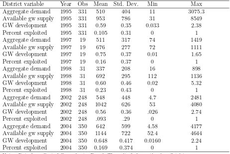
District groundwater data (where the U.S. equivalent of a district is a county) on extraction and recharge from 2004 were provided for 350 districts from 15 states. Obtaining data on groundwater has been our greatest constraint - groundwater assessments are expensive and difficult to undertake and are therefore rarely conducted. We form an unbalanced panel of groundwater data for these districts using groundwater data from 331 districts in 1995, 19 districts in 1997, 31 districts in 1998, 248 districts in 2002 and 350 districts in 2004. Summary statistics on groundwater demand, the replenishable supply, groundwater development and exploitation are provided in Table 1.
In 1998, average district consumption in Madhya Pradesh accounts for 60 percent of the annual replenishable supply and over-exploitation of groundwater occurs in 23 percent of the state’s dis-tricts.7 In 2002, average district consumption amounted to 56 percent of the annual replenishable
groundwater supply. In 23 percent of the 248 districts, groundwater consumption exceeds the replenishable supply. In the 2004 data, average district consumption amounts to 64 percent of
7
the replenishable groundwater supply and 17 percent of the 204 districts are classified as “over-exploited”. Between 2002 and 2004, groundwater development increased by 14 percent and the number of exploited districts grew by 9 percent (panel data is available for 248 districts).
Data collected in 2002 by the Central Groundwater Board of India (CGWB) spatially char-acterize fixed hydrogeological characteristics in the states of Andhra Pradesh, Bihar, Karnataka, Uttar Pradesh, Madhya Pradesh, Maharashtra, Orissa, Tamil Nadu and Rajasthan. Variation in groundwater characteristics is at the district level, where the minimum and maximum depth to the aquifer are calculated as the district mean.
5.2
Electricity data
Electricity data were gathered from three primary sources: “The Annual Report on the Working of State Electricity Boards and Electricity Departments” published by the Power and Energy Division of the Planning Commission between 1992 and 2002, multiple volumes of “Average Electric Rates and Duties in India” published by the Central Electricity Authority and multiple volumes of “Energy”, a publication by the Center for Monitoring the Indian Economy in India.
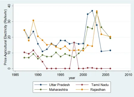
Data on states’ electricity prices, measured in 1986 paise per kilowatt hour (paise/kWh), were collected for the period 1986-2004. The electricity prices captured are average tariffs, measured as the revenues from sale to particular sectors divided by the units sold. Trends in agricultural electricity prices are displayed in Figures 1 and 2. Figure 1 illustrates mean electricity prices over time, showing that between 1995 and 2004 prices have ranged from 9.6 to 20.6 paise. In addition to variation in electricity prices over time, electricity prices also vary across states. The mean electricity price in each state significantly differs from mean electricity prices in at least two other states. In Figure 2, electricity prices are disaggregated by state for a subsample of states. With the exception of Tamil Nadu, prices significantly differ within a state over time. In India, electricity prices also vary by sector with industrial and commercial users paying higher fees. The mean electricity price for agriculture in our sample was 11.3 paise as compared to 103 paise for industrial users.
Table 2 presents descriptive statistics on electricity during the period. Generation and total capacity are captured at a state level and are measured in millions of kW hours. While both generation and capacity have increased substantially during the period, evidence suggests that generation has not increased in line with demand (Tongia, 2004). Transmissions and distribution losses, which reflect both losses due to both technical reasons and theft, have risen substantially over the period examined.
backed out by examining the difference between unit costs and the tariff paid by agricultural users. The subsidy to the agricultural sector increases over the period, from approximately 60 paise per kilowatt hour, to over 80 paise. The subsidy account for approximately 87% of the cost of electricity - on average, the price faced by agricultural users is 13% of the cost of electricity.
5.3
Agricultural production data
District-year level data on agricultural yields comes from two publications at the Ministry of Agriculture - the “Agricultural Situation in India” and the “Area and Production of Principal Crops in India”. In order to decouple the effects of price changes from output changes, we create a Lespeyres volume index of total, water and non-water intensive output using average 1995 prices. Prices were taken from “Agricultural Prices in India”.
Agricultural data include agricultural production in a district-year, individual crop yields, crop acreage and whether or not a crop is grown in a district-year. Data are available for 1995, 1997, 2002 and 2004. Total agricultural production is measured as the sum of production in wheat, rice, cotton, sugar, sorghum, and millet, weighted by the average 1995 market price of these crops. These six crops were chosen due to the widespread availability of data on these crops during the period examined and their prevalence across India. Water-intensive output is measured as the weighted sum of production in sugar, rice and cotton. Rice is grown in 76 percent of the district-years, sugar is grown in 63 percent of the district-years while cotton is grown in 48 percent of the district-years. Sorghum, wheat and millet are defined as non-water intensive crops. Wheat, sorghum and millet were grown in 55, 40 and 38% percent of districts in 1995, respectively. The water intensity of these crops was defined according to their relative levels of water usage, as defined by the FAO. In 1995, 61% of total production was attributable to water intensive crops.
6
Results
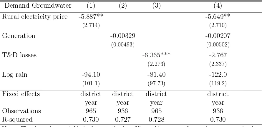
Table 3 reports results from the estimation of equation 9, an OLS model of demand for groundwa-ter. Identification in the model comes from state-year shocks in electricity prices, generation, and transmission and distribution losses, controlling for fixed district unobservables. We report results for the effect of electricity prices on groundwater extraction in column 1. Results for the impact of generation and T&D losses on groundwater extraction are presented in columns 2-3, though we are cautious in interpreting these results due to omitted variables bias.8 We also look at the
effect of electricity prices on groundwater extraction conditional on generation, and transmission and distribution losses (column 4).
8
We find that on average district demand for groundwater decreases by 5.9 million cubic meters with with a 1 paise increase in the price of electricity. Our results suggest that a 25 percent increase in the agricultural price of electricity, where the mean price of electricity is 11.8 paise/kWh, will reduce mean groundwater demand by 16.5 mcm or roughly 2.7 percent. If electricity subsidies were reduced by 10%, where the average subsidy over the duration of the study amounted to 87 paise/kWh, demand for groundwater would decrease by 7.4 percent. It should be noted that while these results suggest a price inelastic demand for groundwater, the source of variation exploited implies that the estimates capture only a short-run elasticity of demand. In the long-term as the area and the crops cultivated responds to changes in the price of groundwater, the demand response is likely to be greater.
When we estimate the effect of one type of electricity subsidy on groundwater extraction, our results suggest that T&D losses and electricity prices are each significant in explaining district demand for groundwater. Once we condition each electricity subsidy on the other electricity subsidies, electricity price is the only subsidy that significantly impacts groundwater extraction. Conditional on other electricity subsidies, a 1 paise increase in electricity prices is predicted to decrease groundwater extraction by 5.6 million cubic meters. This result mirrors that reported in column 1, suggesting that our results are robust to the inclusion of other subsidies.
In Table 3 coefficient estimates on electricity prices may be downward biased since unobserv-ables - the political party in power or the size of a state’s agricultural economy - that may increase groundwater extraction may also be negatively correlated with electricity prices.
To identify the effect of electricity prices on groundwater extraction, we estimate equation 10, a district fixed effects model in which we interact groundwater characteristics with agricultural electricity prices and control for state-year shocks; results are reported in Table 4. In this model we are unable to measure the direct effect of electricity prices on demand for groundwater. Rather we estimate the differential effect of electricity prices on districts with different minimum well depths within a state-year. We find evidence that an increase in electricity prices reduces groundwater extraction relatively more in districts with deeper wells (higher priced groundwater sources). For a district with the mean tube well depth (58 m), we find that a 25 percent increase in the agricultural price of electricity reduces groundwater extraction by 9.67 mcm or 1.61 percent. Our results suggest that a 10% decrease in the average electricity would reduce district groundwater extraction by 4.3 percent.
6.1
Agricultural production
of an OLS model of the value of agricultural output on electricity prices. This model estimates the effect of state-year electricity prices on agricultural revenues within a district, controlling for year shocks. Our results suggest that a 1 paise increase in electricity prices, which approximates an 9 percent price increase, induces a 4.8 percent reduction in agricultural revenues. This finding is both economically and statistically significant, and suggests a large reduction in annual rev-enues should electricity subsidies be reduced. For example, a 25 percent increase in electricity prices would reduce revenues by 13.4 percent and a 10 percent reduction in subsidies would lower revenues by more than one-third.
The magnitude of the estimated impact of electricity prices on agricultural revenues suggests that unobservables that are positively correlated with groundwater extraction may also systemat-ically increase agricultural revenues. For example, fertilizer subsidies, the other dominant agricul-tural subsidy in India, will likely lead to an increase in groundwater extraction and agriculagricul-tural output. To isolate the effect of electricity subsidies (via the channel of groundwater extraction) on agricultural output, we estimate equation 10, an OLS model in which we interact electricity prices with minimum well depth, except now importantly the dependent variable is agricultural production.
Column 2 reports results. Consistent with the predictions in our theoretical model, we find that electricity subsidies led to a significant increase in agricultural revenues. Our results suggest that a 1 paise increase in the price of electricity would cause a 1.77% decrease in agricultural revenues. Compared to column 1, electricity prices have a less substantial impact on agricultural revenues; a 25 percent increase in electricity prices is predicted to reduce agricultural revenues by 5 percent. A 10% reduction in the subsidy would lower agricultural revenues by 13 percent. This evidence suggests that electricity subsidies in India benefited farmers, when benefits are measured as agricultural revenues. However, if we simply estimate the effect of electricity subsidies on agricultural outputs, the stimulus provided by these subsidies will be largely overstated. In fact, the predicted impacts of electricity subsidies in the interaction model are roughly one-third those reported in the simple OLS model.
If we breakdown agricultural revenues by water intensive and non-water intensive crops, we observe significant changes in both water intensive (cols. 3 and 4) and non-water intensive (cols. 5 and 6) crop revenues in response to a change in electricity prices. All things equal, we would expect water intensive crop revenues to be more responsive to electricity prices, since these crops use more water and hence electricity. However, in fact we find that revenues from non-water intensive crops are more sensitive to price changes, dropping by approximately 1.7 percent with a 1 Rs increase in electricity prices (col. 6). In comparison, we observe a 1.4 percent decrease in water intensive revenues in response to a change in electricity prices (col. 4).
crops should increase relative to those of non-water intensive crops. Since we don’t have data on water used by crop, we instead examine yields to estimate whether production per hectare cultivated is responsive to changes in electricity subsidy. This captures whether the amount of water and other complementary inputs fall as electricity subsidies fall.
In Table 6, we report results from the estimation of an OLS model of crop level agricultural yields on electricity prices. In columns 1-3 we show the impact of electricity subsidies on wa-ter intensive crop yields for three crops - cotton, sugar and rice; columns 4-7 report the effect of electricity subsidies on non-water intensive crop yields for wheat, maize, sorghum and millet. Consistent with our theoretical predictions, we find that an increase in electricity prices, signifi-cantly reduces yields for water intensive crops, has no statistically significant impact on maize and wheat while it raises yields on the least water intensive of all the crops, sorghum and millet. Both cotton and rice yields are sensitive to electricity prices. We find a 1.5 percent decrease in cotton yields and 0.55 percent decrease in rice yields with a 1 paise or 9 percent increase in electricity prices.
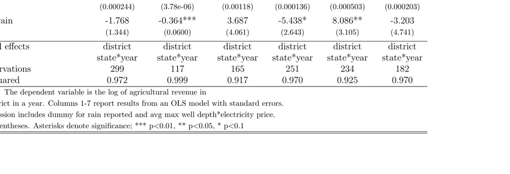
Table 7 displays results from the estimation of an OLS model of crop acreage, our measure of the extensive margin, on electricity prices. Our theoretical model predicts that the fraction of land devoted to the water intensive crop will increase as the price of water decreases. Consistent with our theoretical prediction, we find that when at least 50 percent of the district area is suitable for crop growth, the acreage on which rice grows increases with a decrease in the price of groundwater. A 1 paise increase in electricity prices generates a 0.6 percent decrease in crop acreage devoted to rice. In contrast, we find that when the land is not suitable to the cultivation of rice, there is no impact of electricity (groundwater) prices on rice acreage. We find that cotton and sugar acreage are not responsive to electricity prices.
7
Welfare Effects
The results in the previous section suggest that agricultural users respond to electricity subsidies by increasing groundwater extraction and agricultural output, especially for water intensive crops. This section explores the welfare impacts of electricity subsidies, quantifying the deadweight loss of these subsidies. We specify derived demand for electricity and a long run marginal cost curve, and then estimate the reduced inefficiency from a 10 percent reduction in agricultural electricity subsidies.
7.1
Electricity demand
for a unit of groundwater, given by the interaction of state-year electricity prices and minimum aquifer depth in a district or DAM in
i ∗pEAg,jt, is in units of meter-dollars. A consequence of our
measure of groundwater prices is that the consumer surplus and deadweight loss estimated using derived demand for groundwater do not have a monetary interpretation. To convert aquifer depth into a price, we would need to specify a relationship between aquifer depth and electricity usage, and groundwater extraction and electricity usage. Instead of making this conversion, we rely on derived demand for electricity to quantify the deadweight loss.
Suppose farmers have a log-linear derived demand for electricity, (E|λt, γj) = α0(DAM in ∗
pE
Ag,jt, DAM ax∗pEAg,jt|λt, γi)α1 where we condition on state and year unobservables. We can estimate
derived agricultural demand for electricity in state j and year t as
lnEjt =α0+α1pEAg,jt+λt+γj +ηjt+ujt (13)
where DAmin and DAmax are absorbed in the state fixed effect. The quantity of electricity
consumed, Ejt is measured as annual electricity sales for agriculture; pEAg,jt measures the
state-year price of agricultural electricity; λt captures year shocks; ηjt denotes state trends. The error
structure includes γj, a state fixed effect, andujt, an idiosyncratic error term that is clustered at
the state. Crop prices and the land endowment are captured in the year and state fixed effects.9
Table 8 reports results. In column 1, we do not control for state trends and in column 2, we report results from the estimation of equation 13. We use electricity data from 15 states between 1986 and 2005. As expected demand for electricity is responsive to state electricity prices, though electricity demand is inelastic in the short-run. Our results suggest that a 10 percent increase in electricity prices reduces demand for electricity by 1.2 when we omit state trends and by 0.6 percent once we control for state trends. The price inelasticity of demand is unsurprising given (i) that we are analyzing demand using year to year variation and (ii) the magnitude of the existing subsidies on electricity.
7.2
Efficiency Costs
To measure the deadweight loss generated by this subsidy, we perform a simple counterfactual and estimate electricity sales under the current price structure and if the electricity subsidy was reduced by 10 percent.
We assume that the long-run marginal cost of electricity is equal to the average cost of electricity across-all state years; MC=82 paise per kwh. The electricity subsidy equals 70.15 paise per kwh, the average difference between the unit cost of electricity and the price of electricity, for the 189 state-years in which both prices are observed.
One limitation in our inefficiency estimate is that we cannot calculate the deadweight loss of
9
switching from a policy in which electricity is priced at the marginal cost to one in which electricity is priced at the status-quo. Rather we predict the reduction in deadweight loss (efficiency gain) if there was a 10% reduction in the subsidy. We calculate the effect of a 10 percent reduction rather than a complete removal of the subsidy due to concerns about out of sample predictions. In our sample, the average per unit cost of electricity is 82 paise per kWh, though farmers on average only pay 11.8 paise per kWh. There is no overlap between agricultural prices and the unit cost of supply; electricity prices for agriculture range between 0 and 36.4 paise whereas the unit cost of supply ranges between 47 and 148 paise. Since there are no observations in which the agricultural price equals the unit cost of electricity, we cannot reasonably predict the impact of unit cost pricing on agricultural revenues. By contrast if we reduce the subsidy by 10%, the calculated price of electricity overlaps with the observed price of electricity in all states in the study with the exception of two.
When agricultural users face a price of electricity equal to pe, the deadweight loss from the
subsidy is calculated as,
DW L(pe) = (mc−pe)(E(pe)−E(mc))− Z mc
pe
(E(p)dp) (14)
where mc is defined as 90% of the current electricity subsidy. First, we calculate the deadweight loss for each state under the current subsidy. We then aggregate the deadweight loss of each state fo find the total efficiency gains of a 10% reduction in agricultural electricity subsidies.
References
[1] Besley, Timothy and Burgess, Robin, (2002), “The Political Economy of Government Responsiveness: Theory and Evidence from India,”The Quarterly Journal of Economics,
117(4):1415-1451.
[2] Birner, Regina, Surupa Gupta, Neera Sharma and Nethra Palaniswamy, (2007), “The Political Economy of Agricultural Policy Reform in India: The Case of Fertilizer Supply and Electricity Supply for Groundwater Irrigation”, New Delhi, India: IFPRI
[3] Briscoe, John and Malik, R.P.S., (2006), India’s Water Economy: Bracing for a Turbulent Future, New Dehi, India: Oxford University Press.
[4] De Janvry, Alain and Sadoulet, Elizabeth, (2006), “Making Conditional Cash Transfer Pro-grams More Efficient: Designing for Maximum Effect of the Conditionality,”The World Bank Economic Review 20(1):1-29.
[5] Domenico, P.A., Anderson, D.V., and Case, C.M., (1968), “Optimal Ground-Water Mining,”
Water Resources Research, 4(2): 247-255.
[6] Dubash, Navroz K., (2007), “The Electricity-Groundwater Conundrum: Case for a Political Solution to a Political Problem,” Economic and Political Weekly, 45-55.
[7] Dubash, Navroz K. and Rajan, Sudhir Chella, (2001), “Power Politics: Process of Power Sector Reform in India,” Economic and Political Weekly 36(35):3367-3387.
[8] Ghosh, Arkadipta, (2006), “Electoral Cycles in Crime in a Developing Country: Evidence from the Indian States,” working paper.
[9] Gulati, Ashok, (1989), “Input Subsidies in Indian Agriculture: A Statewise Analysis,” Eco-nomic and Political Weekly 24(25):57-65.
[10] Gulati, Ashok and Narayanan, S., (2000), “Demystifying Fertiliser and Power Subsidies in India”, Economic and Political Weekly, 35(10):784-794.
[11] Gulati Ashok and Sudha Narayanan (2003), The Subsidy Syndrome in Indian Agriculture, New Delhi, India: Oxford University Press.
[12] Kremer, Michael, (2003), “Randomized Evaluations of Educational Programs in Developing Countries: Some Lessons,” The American Economic Review 932:102-106.
[14] Martin, William E., and Archer, Thomas, (1971), “Cost of Pumping Irrigation Water in Arizona: 1891 to 1967,” Water Resources Research 7(1): 23-31.
[15] McKenzie, Dave and Ray, I., (2004), “Household Water Delivery Options in Urban and Rural India”, Prepared for 5th Stanford Conference on Indian Economic Development, June 3-5, 2004.
[16] Miguel, Edward and Kremer, Michael, (2004), “Worms: Identifying Impacts on Education and Health in the Presence of Treatment Externalities,” Econometrica 72(1):159-217.
[17] Modi, Vijay (2005), “Improving Electricity Services in Rural India”, Working Paper No. 30. Center on Globalization and Sustainable Development.
[18] Scheierling, S. M., Loomis, J.B., and Young R. A., (2006), “Irrigation water demand: A meta-analysis of price elasticities”, Water Resources Research 42 doi:10.1029/2005WR004009.
[19] Schultz, T. Paul, (2004), “School Subsidies for the Poor: Evaluating the Mexican Progresa Poverty Program,” Journal of Development Economics 74:199-250.
Table 1: Summary Statistics on Supply and Demand for Groundwater
District variable Year Obs Mean Std. Dev. Min Max
Aggregate demand 1995 331 510 404 11 3075.3
Available gw supply 1995 331 953 786 31 8549
GW development 1995 331 0.59 0.35 0.033 2.38
Percent exploited 1995 331 0.105 0.31 0 1
Aggregate demand 1997 19 511 317 74 1419
Available gw supply 1997 19 676 277 72 1111
GW development 1997 19 0.75 0.37 0.01 1.65
Percent exploited 1997 19 0.16 0.37 0 1
Aggregate demand 1998 31 337 208 16 898
Available gw supply 1998 31 692 295 112 1136
GW development 1998 31 0.60 0.46 0.02 5.32
Percent exploited 1998 31 0.23 0.43 0 1
Aggregate demand 2002 248 548 448 4.7 2481
Available gw supply 2002 248 1042 626 53 4080
GW development 2002 248 0.56 0.36 .026 2.74
Percent exploited 2002 248 .093 .29 0 1
Aggregate demand 2004 350 642 599 4.58 4177
Available gw supply 2004 350 1144 722 52.4 4644 GW development 2004 350 0.648 0.417 0.0160 2.24
Percent exploited 2004 350 0.169 0.374 0 1
Notes: Data from Central Groundwater Board. The unit of observation is a district.
Table 2: Summary Statistics on Electricity Prices and Capacity
District variable Year States Districts Mean Std. Dev. Min Max Agricultural Electricity Price 1995 14 331 9.41 404 0 22.13 Industrial Electricity Price 1995 14 331 87.32 786 31 112.71
Generation 1995 14 331 14082 1952 2340 35335
Subsidy 1995 14 331 60.05 12.59 35.39 90.68
Agricultural Electricity Price 1997 1 19 7.43 - -
-Industrial Electricity Price 1997 1 19 107.01 - -
-Generation 1997 1 19 21303 - -
-Subsidy 1997 1 19 67.75 - -
-Agricultural Electricity Price 1998 1 31 2.09 - -
-Industrial Electricity Price 1998 1 31 126.25 - -
-Generation 1998 1 31 17057 - -
-Subsidy 1997 1 19 73.95 - -
-Agricultural Electricity Price 2002 9 197 10.91 13.14 0 3075.3 Industrial Electricity Price 2002 9 197 99.57 47.67 0 8549
Generation 2002 9 197 18552 12309 2608 2.38
Subsidy 2002 9 197 88.95 15.51 57.24 112.61
Notes: The unit of observation is a state, the number of districts examined is given in column 4. Electricity prices and subsidies are measured in 1986 paise. Electricity generation are measured in million kilowatt hours. Electricity subsidies are measured as the difference between the electricity price and the unit cost.
Table 3: OLS models of demand for groundwater
Demand Groundwater (1) (2) (3) (4)
Rural electricity price -5.887** -5.649**
(2.714) (2.710)
Generation -0.00329 -0.00207
(0.00493) (0.00502)
T&D losses -6.365*** -2.767
(2.273) (2.337)
Log rain -94.10 -81.40 -122.0
(101.1) (97.73) (119.2)
Fixed effects district district district district
year year year year
Observations 965 936 965 936
R-squared 0.730 0.727 0.728 0.730
Table 4: OLS model of demand for groundwater with interaction
Groundwater extraction exploited critical -75% Elec price*min well depth -0.0597* -2.54e-07 -1.76e-05
(0.0302) (4.10e-05) (3.39e-05)
Log rain 157.4 -0.000788 0.374
(109.4) (0.0299) (0.296)
Fixed effects district district district
state*year state*year state*year
Observations 551 551 910
R-squared 0.665 0.654 0.814
Notes: The dependent variable is the quantity in million cubic meters of groundwater extraction by a district in a year. Columns 1-5 report results from an OLS model with standard errors.
Regression includes dummy for rain reported and avg max well depth*electricity price. in parentheses. Asterisks denote significance; *** p<0.01, ** p<0.05, * p<0.1
Table 5: OLS model of agricultural production
(1) (2) (3) (4) (5) (6)
Value agricultural product All crops All crops H20 intensive H20 intensive Non-H20 intensive Non-H20 intensive
Elec price -0.0480*** -0.0521*** -0.0463***
(0.00571) (0.00599) (0.00496)
Elec price*min well depth -0.000307*** -0.000245*** -0.000297***
(5.66e-05) (5.26e-05) (0.000101)
Log rain 0.106 -0.252 0.135 -0.231 -0.609 -1.893***
(0.471) (0.446) (0.493) (0.452) (0.452) (0.468)
Fixed effects district district district district district district
year state*year year state*year year state*year
Observations 718 415 717 415 673 397
R-squared 0.935 0.991 0.940 0.992 0.977 0.991
Notes: The dependent variable is the log of agricultural revenue in
a district in a year. Columns 1-7 report results from an OLS model with standard errors. Regression includes dummy for rain reported and avg max well depth*electricity price. in parentheses. Asterisks denote significance; *** p<0.01, ** p<0.05, * p<0.1
Table 6: OLS model of agricultural yields
(1) (2) (3) (4) (5) (6) (7)
Water Intensive Non-Water Intensive
Yields Cotton Sugar Rice Wheat Maize Sorghum Millet
Elec price*min well depth -0.000253*** -5.86e-07 -8.79e-05*** -3.03e-05 -4.32e-05 3.98e-05*** 0.000200***
(5.64e-05) (1.45e-05) (1.76e-05) (1.95e-05) (5.70e-05) (7.77e-05) (6.09e-05)
Elec price*max well depth 0.000209** 5.28e-05* -3.91e-05 -4.41e-05 6.23e-07 -1.28e-05 -8.53e-05*
(8.01e-05) (2.97e-05) (3.47e-05) (4.77e-05) (5.29e-05) (1.97e-05) (4.12e-05)
Fixed effects district district district district district district
state*year state*year state*year state*year state*year state*year state*year
Observations 225 390 414 321 356 300 185
R-squared 0.858 0.978 0.925 0.942 0.896 0.756 0.923
Notes: The dependent variable is the log of agricultural revenue in
a district in a year. Columns 1-7 report results from an OLS model with standard errors.
Regression includes log rainfall, dummy for rain reported and avg max well depth*electricity price. in parentheses. Asterisks denote significance; *** p<0.01, ** p<0.05, * p<0.1
Table 7: OLS model of crop area, by agro-climatic suitability to the crop
(1) (2) (3) (4) (5) (6)
Area crop cultivated Rice Rice Cotton Cotton Sugar Sugar
Not Suitable Suitable Not Suitable Suitable Not Suitable Suitable
Elec price*min well depth 0.000202 -0.000103*** -0.00125 5.50e-05 -0.000613 4.51e-05
(0.000244) (3.78e-06) (0.00118) (0.000136) (0.000503) (0.000203)
Log rain -1.768 -0.364*** 3.687 -5.438* 8.086** -3.203
(1.344) (0.0600) (4.061) (2.643) (3.105) (4.741)
Fixed effects district district district district district district
state*year state*year state*year state*year state*year state*year
Observations 299 117 165 251 234 182
R-squared 0.972 0.999 0.917 0.970 0.925 0.970
Notes: The dependent variable is the log of agricultural revenue in
a district in a year. Columns 1-7 report results from an OLS model with standard errors. Regression includes dummy for rain reported and avg max well depth*electricity price. in parentheses. Asterisks denote significance; *** p<0.01, ** p<0.05, * p<0.1
Table 8: Demand for electricity
Log Ag Electricity Sales (1) (2)
Log(Ag electricity price) -0.121 -0.0611** (0.0708) (0.0273)
Fixed effects state state
year year
Observations 201 201
R-squared 0.762 0.928
Number of state 14 14
Notes: The dependent variable is electricity sales in millions of kwh in a state year. Columns 1-2 report results from an OLS model with standard errors clustered at the state in parentheses. State year trends are included in column 2.
Asterisks denote significance; *** p<0.01, ** p<0.05, * p<0.1