An Innovative Heuristic in Multi-Item Replenishment Problem for
One Warehouse and
N
Retailers
Yugowati Praharsi
1*, Yessica Nataliani
1, Hui-Ming Wee
2Abstract: Joint replenishment problem (JRP) is a type of inventory model which aims to minimize the total inventory cost consisting of major ordering cost, minor ordering cost and inventory holding cost. Different from previous papers, this study considers one warehouse, multi items and N retailers. An innovative heuristic approach is developed to solve the problem. In this paper, we consider a multi echelon inventory system and seek to find a balance between the order cost and the inventory holding costs at each installation. The computational results show that the innovative heuristic provides a near exact optimal solution, but is more efficient in terms of the computational time and the iteration number.
Keywords: Inventory, joint replenishment problem (JRP), single warehouse multiple retailers, multi-items, heuristic.
Introduction
In recent years, new methods are developed to fulfil customers need in retail business more efficiently. One of the methods is the joint replenishment problem (JRP). JRP is a method to replenish multi-items from a single supplier or warehouse. The JRP consists of major and minor order costs.
JRP is divided into two strategies, i.e. direct and indirect grouping. In the direct grouping strategy (DGS), items are classified into different group with each group jointly replenished. In the indirect grouping strategy (IGS), all replenishments occur at constant intervals of a common time period. The IGS outperforms of DGS in higher major ordering cost (Eijs et al. [1]). In this research, the IGS with strict cycle policy is used where at least one item is ordered at every replenishment opportunity.
In the JRP for single echelon level, Praharsi et al. [2] developed an innovative heuristic to solve the extension of traditional JRP for centralized and decentralized replenishment policies at the retailer. The innovative heuristic can be implemented in deterministic and stochastic demands. Hoque [3] extended the traditional JRP model with storage and transport capacities and budget constraints. Zhang
et al. [4] also extended the traditional JRP with complete backordering and correlated demand.
1 Department of Information Technology, Satya Wacana Christian University, Jl. Diponegoro 52-60, Salatiga 50711, Indonesia. Email: [email protected];[email protected] 2 Department of Industrial and System Engineering, Chung Yuan Christian University, Chung Pei Rd. 200, Chung Li, 32023, Taiwan ROC. Email: [email protected]
*Corresponding author
Wang et al. [5] discussed joint replenishment under interdependence of minor ordering costs. Moon et al.
[6] developed joint replenishment and consolidated freight delivery models for a warehouse.
In the JRP for two echelon levels, Chen and Chen [7] studied centralized and decentralized decision models with one manufacturer and one retailer. Chen and Chen [8] also studied the effect of supply chain improvements based on the joint replenishment with a channel coordination practice between a manu-facturer and a retailer. Hsu [9] presented JRP for a central factory and multiple satellite factories in order to take the advantage of economic of scale in the freight cost. Tsao and Sheen [10] discussed the variations of supplier’s credit policy and freight transport discounts from individual and channel perspectives between supplier and retailer.
In the JRP for multi echelon levels, Tsao [11] presented multi-echelon multi-item channels in which retailer determined the promotional effort to the customers and the joint replenishment cycle while supplier determined the credit period. Cha et al. [12] studied more flexible policy for the joint replenishment and delivery scheduling of a ware-house with N retailers system. The warehouse has the flexibility in terms of the joint replenishment to the suppliers and individual distribution policies to the retailers. This paper extends the traditional JRP for one warehouse N retailers into more practical issue that the retailers can place an order regardless of the replenishment time of the warehouse.
the RAND method [15]. Later, Goyal and Deshmukh [16] modified the RAND method to get a tight lower bound that was helpful and it outperformed the original RAND. A comprehensive review of several algorithms approaches used in JRP can be found in Khouja and Goyal paper [17]. In 2007, Nilsson et al.
[18] introduced a new heuristic that is based on the balancing the replenishment and the inventory holding costs for different items in an iterative procedure. It is shown that the method outperforms the modified RAND. Nilsson’s heuristic (Nilsson et al., [18]) is implemented in the traditional JRP model for single echelon. Moreover, the traditional JRP has been studied extensively for single echelon, two echelon, and multi echelon levels. In this study, we will develop Nilsson’s heuristic for multi echelon supply chain.
Generally, the warehouse determines the number of replenishment time to the retailers or from the suppliers. An example of this case is the way of the agent distributes the LPG gas to the retailers in Indonesia. In practice, retailers face some fluctuating demands. Therefore, the retailer’s flexibility to place an order should be considered. The characteristic that a retailer can place an order regardless of the replenishment time of the warehouse is important because a retailer could have a greater respon-siveness of the dynamic market demand and have the flexibility in the number of replenishment. This characteristic significantly affects the order decisions of a retailer.
The first objective of this study is to develop a joint replenishment model for one warehouse N retailers that provide flexibility for retailers to place an order from the warehouse. Then, we propose an algorithm to determine the best solution to minimize costs. We use a similar idea of integer ratio policy that is developed by Nilsson et al. [18] and modified the policy to accommodate multi echelon level. This policy balances the replenishment order cost and the inventory holding cost for different items iteratively in all retailers. The cost will be higher when the ratio is further from one. It follows EOQ model for individual items without safety stock. The result of these innovative heuristic will be compared with the exact optimal solution by LINGO software. It is expected that the innovative heuristic solution will be near to the exact optimal solution. This study also extends the Abdul-Jalbar et al. [19] paper in which the JRP concept is applied for multi-items.
The remainder of the paper is organized as follows: Section Methods describes the proposed model for one warehouse N retailer problem in classical model.
Warehouse
R1
R2
RN
Figure 1. One warehouse and N retailers system
t0
t1
t2
W
a
re
h
o
u
se
R2 R1
f1=3
f2=2
R3
t3
f3=1/2
Figure 2. Replenishment system for one warehouse N retailers
In Results and Discussion, we conduct a numerical example and some experiments. Finally, concluding remarks and future research are presented in the last section.
Methods
Modeling Process
The supply chain system of one warehouse N
retailers can be illustrated as in Figure 1.
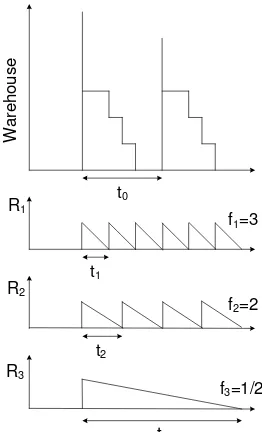
The warehouse orders from an outside supplier to replenish retailers demand for multi-items. The retailers can place an order regardless of the replenishment time of the warehouse. It can be illustrated by Figure 2.
Figure 2 presents an example of inventory level for one warehouse with three retailers where
then { }. The warehouse has invent-tory for retailers when replenishment time at retailer is smaller than the one at the warehouse or
, for R = 1, …, N. The parameters of the problem are:
: major ordering cost associated with each replenishment at the warehouse ($/order) : minor ordering cost incurred if item i is
ordered in a replenishment by a warehouse : time between successive replenishments at
the warehouse (weeks)
: holding cost of item i at the warehouse ($/unit/weeks)
: demand for item i at retailer R (units/ weeks)
: the number of replenishment for retailer R
during
: major ordering cost associated with each replenishment at retailer R ($/order) : minor ordering cost incurred if item i is
ordered in a replenishment by retailer R
: time interval between successive replenish-ment of item i at retailer R
: time between successive replenishments at retailer R
: holding cost of item i at retailer R ($/unit/weeks)
: the ratio between the two cost for item-i at retailer R (i.e. replenishment cost/holding cost)
The decision variables are the following:
: the integer number of intervals that the replenishment quantity of item i will last, for R= 1, …,N and i= 1, …., m
: time between successive replenishments at the warehouse (weeks)
TC : total costs at warehouse and retailers consist of order costs and inventory holding cost
Assumptions used in this study are: (1) demand rate for each item is constant, (2) retailers replenish stocks from warehouse based on the EOQ, subject to a major order cost for placing an order and a minor order cost for each specific item ordered, (3) backor-dering costs are not considered, (4) a strict cycle policy is used in which at least one item is ordered at every replenishment opportunity, or
The order cost at the warehouse consists of major order cost and minor order cost. The average order cost at the warehouse can be formulated as ⁄
⁄ .
The inventory holding cost at the warehouse occurs only when or Moreover, the average inventory holding cost at the warehouse can be formulated as ∑ ∑ for
The order cost at retailers also consists of major order cost and minor order cost for each specific item incurred. The average order cost at retailers can be
presented as
∑
∑
∑
, where
and .
The inventory holding cost at retailers involves all specific items in each retailer. The average holding cost at retailers can be written as ∑ ∑ The average total cost for the system can be established as follows:
∑ ∑ ∑
∑ ∑ ∑ ∑ ∑ (1)
Remodel TC in terms of , one has:
∑ ∑ ∑ ( ⁄ )
∑ ∑ ∑ ∑ ∑ (2)
The second partial derivative of TC with respect to
is ∑ ∑ ∑
.
Therefore, the cost function is convex at . Taking the first partial derivative of TC with respect to , and setting it as equal to 0 yields the optimal time interval, , that minimizes (2) with a given set of
as follows:
√
( ∑ ∑ ∑ ∑
)
∑ ∑ ( )
∑ ∑
(3)
Substituting optimal into (2) gives the total cost function, which depends only on the set of values. It is given as in equation (4)
√ ∑ ∑ ∑ ∑ ∑ ∑
∑ ∑
The replenishment cost and inventory holding cost for item i can be written as follows:
(5)
(6)
Dividing (5) by (6) resulting the ratio between the two costs for item i:
(7)
An Innovative Heuristic Procedure
Nillsson et al. [18] presented a heuristic method to solve a JRP model for single echelon. In this study, this heuristic has been modified and reworked to better suit the JRP for multi echelon, but still has the same basic principle to balance the replenish-ment cost and the holding cost for each individual item.
The JRP concept is the same as the traditional EOQ for an individual item. The ratio between the replenishment/order cost and the inventory holding cost is equal to one which excludes safety stock. The closer the individual ratio approaches to one, the better the solution.
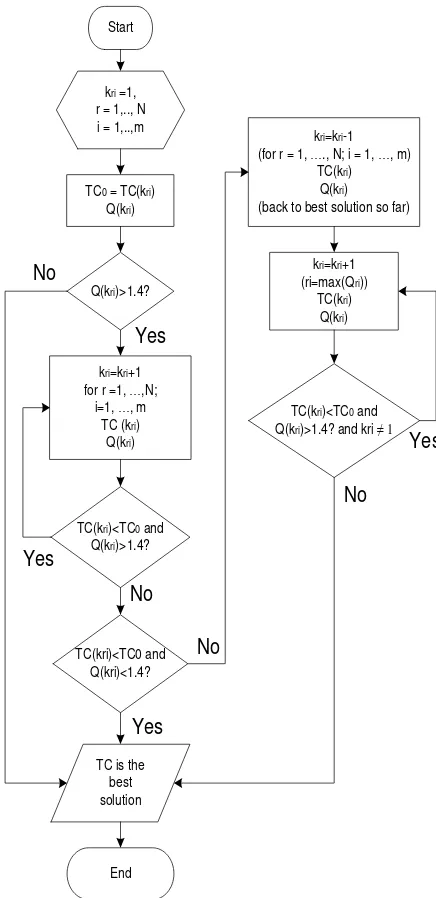
We can adjust the ratio closest to one by an innovative heuristic procedure. This procedure balances the order cost and inventory holding costs for different items in each retailer iteratively. There are two steps needed in this heuristic method. The first step is setting the values to one (all items are replenished every time interval). Subsequently, tracking the ratios and the total cost changes as the replenishment frequencies are updated. The detail of an innovative heuristic procedure is presented in Figure 3.
The steps are described below:
1. Set all values of to 1, and compute the total cost for the initial solution
2. Compute and increase the values of by one for all items with ratios higher than 1.4. 3. Calculate the total cost. Repeat until all ratios are
below 1.4 or the total cost starts to increase. 4. If all ratios are below 1.4, then we have derived
the best solution for the total cost.
5. If the total cost starts to increase, the best solution is the previous iteration.
6. Choose the highest from all retailers and items. Then increase value by one for the Rth retailer and ith item.
7. Calculate the total cost and ratios. Repeat this until all ratios are below 1.4. If there is ,
Start
kri =1, r = 1,.., N i = 1,..,m
TC0 = TC(kri) Q(kri)
Q(kri)>1.4?
kri=kri+1 for r =1, …,N;
i=1, …, m TC (kri)
Q(kri)
Yes
TC(kri)<TC0 and Q(kri)>1.4?
Yes
TC(kri)<TC0 and Q(kri)<1.4?
No
TC is the best solution
End
Yes
kri=kri-1 (for r = 1, …., N; i = 1, …, m)
TC(kri) Q(kri) (back to best solution so far)
No
kri=kri+1 (ri=max(Qri))
TC(kri) Q(kri)
TC(kri)<TC0 and Q(kri)>1.4? and kri ≠ 1
Yes
No
No
Figure 3. Flowchart of an innovative heuristic procedure
The value 1.4 is chosen because it produces the lowest error (Nilsson et al. [18]). Nilsson et al. [18] already tested for 48,000 benchmark problems with the value of ratios ranging from 1.0 to 2.0.
Results and Discussions
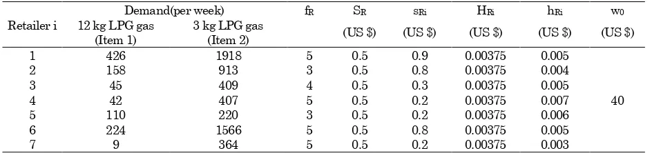
A numerical example is presented in Table 1. The example consists of one warehouse and seven retailers. There are 2 items where the demand rate, the holding cost, the major and minor replenishment costs, and the number of replenishment time during at the retailers are known. The data is a part of real case from LPG gas agent in Indonesia. The type of LPG gas consists of 12 kg and 3 kg. In this case there is no minor ordering cost incurred from the warehouse to the supplier ( ).
There are three types of decision variables in this numerical example: a) time between successive replenishment at the warehouse b) the integer number of intervals, where R = 7, and i = 2; and c) costs at the warehouse and retailers (TC*). Because we have 16 variables, there is a need to solve it by heuristic procedure.
Case Study
Table 2 shows the results for innovative heuristic method and the exact optimal solution by Lingo 11.0 software. The approach employed by Lingo 11.0 is branch-and-bound, called by its non-linear global solver. For all the numerical examples in this paper, Lingo 11.0 can yield the exact optimal solutions. Therefore, the solutions derived from Lingo 11.0 can be used as the benchmarks for evaluating the opti-mality of the heuristic algorithm.
Table 2. Results from the initial data Method
Variable Innovative heuristic Lingo Item 1 Item 2 Item 1 Item 2
kRi
R1 2 1 2 1
R2 2 1 2 1
R3 3 1 3 1
R4 3 1 2 1
R5 1 1 1 1
R6 3 1 3 1
R7 8 2 8 2
TC 65.999 65.994
t0 2.286 2.290
The total cost system for the warehouse and 7 retailers is $65.999 and $65.994 for innovative heuristic and Lingo, respectively. Time between suc-cessive replenishments at the warehouse is 2.286 and 2.290 for innovative heuristic and Lingo, respectively. The integer number of time interval between successive replenishment of item i at retailer R in innovative heuristic is the same as the exact optimal solution, except at . The results of innovative heuristic are very close to the exact optimal solution. Based on those results, the ware-house could manage the replenishment of items to the retailers in order to minimize the total cost system.
Computational Results
This section provides a set of randomly generated numerical examples to illustrate the average effectiveness of innovative heuristic. We generate 100 instances for each N = 5, 15, 30 and m = 5, 15, 30. The values of wi, Hi, sRi, and hRiare taken from a
uniform distribution U[1, 500]. The values of DRi are taken from uniform distributions U[1, 1000]. W0 and
SR are set to 1000 and 0.1 w0, respectively. For each
instance, we compute both the innovative heuristic (Inv) and the innovative heuristic with modified Quotient (Mq). The latter approach increases the value according to the highest quotients in each retailer for all items. The results are summarized in Table 3.
Table 3. Comparison between the innovative heuristic and modified quotient approach
N m CInv = CMq CInv<CMq CInv>CMq
5 5 90 9 1
15 83 13 4
30 87 8 5
15 5 83 16 1
15 73 20 7
30 68 23 9
30 5 73 21 6
15 83 13 4
30 67 22 11
Total average 78.56 16.11 5.33 Table 1. Initial data
Retailer i
Demand(per week) fR SR sRi HRi hRi w0
12 kg LPG gas (Item 1)
3 kg LPG gas
(Item 2) (US $) (US $) (US $) (US $) (US $)
1 426 1918 5 0.5 0.9 0.00375 0.005
40
2 158 913 3 0.5 0.8 0.00375 0.004
3 45 409 4 0.5 0.3 0.00375 0.005
4 42 407 5 0.5 0.2 0.00375 0.007
5 110 220 3 0.5 0.2 0.00375 0.006
6 224 1566 5 0.5 0.8 0.00375 0.005
Table 4. Average gaps, maximum gap, and standard deviations of these gaps obtained when the Innovative Heuristic (CInv) is compared with the modified quotient (CMq)
N m
CInv<CMq CInv>CMq Avg
(gap) Max (gap)
Dev (gap)
Avg (gap)
Max (gap)
Dev (gap) 5 5 0.009 0.452 0.049 0.000 0.028 0.003 15 0.019 0.466 0.063 0.002 0.066 0.010 30 0.012 0.430 0.056 0.007 0.401 0.043 15 5 0.024 0.356 0.067 0.001 0.102 0.010 15 0.027 0.338 0.072 0.005 0.155 0.021 30 0.017 0.297 0.042 0.003 0.129 0.014 30 5 0.014 0.289 0.044 0.003 0.123 0.015 15 0.013 0.538 0.059 0.002 0.058 0.009 30 0.012 0.246 0.034 0.005 0.171 0.022
Max (gap) 0.538 0.401
Average 0.016 0.054 0.003 0.016
Table 5. Comparison between costs obtained using both heuristics and the exact optimal solution
N m Average gap (%) CInv vs. Copt
Average gap (%) CMq vs. Copt
2 2 0.078 0.083
2 4 0.135 0.141
5 5 0.213 0.222
7 6 0.272 0.286
7 7 0.300 0.316
In Table 3 the first and second column represent the number of retailer and item, respectively. In the third column, we show the number of problems where both the innovative heuristic and modified quotient provide the same solution. The fourth and the fifth column contain the number of instances where the innovative heuristic computes better and worse policies than the modified quotient approach, respectively. As you can see, in 16.11% of the instances the innovative heuristic provides better solutions than those given by the modified quotient procedure, and in 78.56% both methods compute the same solution. Therefore, only in 5.33% does our innovative heuristic provide worse solutions. Hence, we can conclude that in some cases the innovative heuristic is more effective than the modified quotient approach.
In Table 4, we compare the costs of the policies provided by the innovative heuristic procedure with
the costs of the policies given by the modified approach. In particular, for a given number of retailers and items, N and m, respectively, Table 4 shows the average gaps, avg (gap), the maximum gaps, max(gap), and the standard deviations of these gaps, Dev (gap). Notice that all these values are presented in percent. In columns 3-5 we report the results obtained when CInv<CMq, and in columns 6-9 the values obtained when CInv>CMq (Table 4). To compare the amount in the cost differences and not only the number of cost differences we do the following complementary calculations.
In case of CInv<CMq, we compute
Otherwise, if CInv>CMq, we calculate
As can be seen in Table 4, all average gaps are smaller than 0.02%, all maximum gaps smaller than 0.6%, and all standard deviations smaller than 0.06%.
We use the exact optimal solution to compare the effectiveness of the policies provided by the innovative heuristic and by the modified quotient approach. The exact optimal solutions are obtained by Lingo 11.0. For each instance we compute
. In Table 5, we report for each
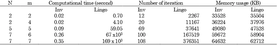
combination of N and m the average percentages. These results show that the innovative heuristic provides closer solutions to the exact optimal solution than the modified quotient approach. All the test problems are solved on a computer with 1.8 GHz CPU and 2.00 GB memory. For different number of retailers and items, the computational times and the number of iterations consumed by the Lingo 11.0 software and Innovative heuristic are shown in Table 6.
From Table 6, it is observed that the computational time of the exact optimal solution provided by Lingo 11.0 increases rapidly as the number of retailers and items increases. However, the computational time consumed by the innovative heuristic is at most a few seconds for all the numerical examples, which proves that the innovative heuristic is very efficient. The efficient performance of innovative heuristic is Table 6. CPU times, number of iteration and memory usage consumed by the Innovative heuristics and Lingo 11.0
N m Computational time (second) Number of iteration Memory usage (KB)
Inv Lingo Inv Lingo Inv Lingo
2 2 0.02 0.70 12 2267 33528 35504
2 4 0.02 4.10 20 11167 36224 37976
also supported by the number of iteration. For the memory usage consumed by the innovative heuristic and Lingo, it shows a slightly different.
Conclusion
Limitation and Future Work
In this paper, a multi-item JRP model for multi echelon inventory system is developed. The retailers can place an order regardless of the replenishment time of the warehouse to the supplier. This characteristic significantly affects the order decisions of a retailer. We developed an innovative heuristic algorithm to solve the model. In this paper, we consider a multi echelon inventory system and seek to find a balance between the order cost and the inventory holding costs at each installation. The computational results show that the innovative heuristic provides near exact optimal solution but is more efficient in terms of the computational time and the iteration number. The innovative heuristic can be used as an alternative for solving JRP multi echelon efficiently. The finding also gives insight to the retail manager and agent because they can determine successful replenishment time for each item. This leads to higher customer satisfaction and increased profits. In this study, we use LINGO software for student version with limited variables. Future research can focus on a more general inventory/distribution system with several ware-houses and retailers.
References
1. Eijs, M. J. G. V., Heuts, R. M. J., and Kleijnen, J. P. C., Analysis and Comparison of Two Stra-tegies for Multi-Item Inventory Systems with Joint Replenishment Costs, European Journal of Operational Research, 59, 1992, pp. 405-412. 2. Praharsi, Y., Purnomo, H. D., and Wee, H.-M.,
An Innovative Heuristic for Joint Replenish-ment Problem with Deterministic and Sto-chastic Demand, International Journal of Electronic Business Management, 8, 2010, pp. 223-228.
3. Hoque, M. A., An Optimal Solution Technique for the Joint Replenishment Problem with Storage and Transport Capacities and Budget Constraints, European Journal of Operational Research, 175, 2006, pp. 1033-1042.
4. Zhang, R., Kaku, I., and Xiao, Y., Model and Heuristic Algorithm of the Joint Replenishment Problem with Complete Backordering and Correlated Demand, International Journal of Production Economics, 139, 2012, pp. 33-41. 5. Wang, L., He, J., Wu, D., and Zeng, Y. R., A
Novel Differential Evolution Algorithm for Joint
Replenishment Problem under Interdependence and Its Application, International Journal Production Economics, 135, 2012, pp. 190-198. 6. Moon, I. K., Cha, B. C., and Lee, C. U., The Joint
Replenishment and Freight Consolidation of a Warehouse in a Supply Chain, International Journal of Production Economics, 133, 2011, pp. 344-350.
7. Chen, J. M., and Chen, T. H., The Multi-item Replenishment Problem in a Two-Echelon Sup-ply Chain: The Effect of Centralization versus Decentralization, Computers and Operations Research, 32, 2005, pp. 3191-3207.
8. Chen, T. H., and Chen, J. M., Optimizing Supply Chain Collaboration Based on Joint Replenish-ment and Channel Coordination, Transportation Research Part E, 41, 2005, pp. 261-285.
9. Hsu, S. L., Optimal Joint Replenishment Decisions for a Central Factory with Multiple Satellite Factories, Expert Systems with Appli-cations, 36, 2009. pp. 2494-2502.
10. Tsao, Y. C., and Sheen, G. J., A Multi-Item Supply Chain with Credit Periods and Weight Freight Cost Discounts, International Journal Production Economics, 135, 2012, pp. 106-115. 11. Tsao, Y. C., Managing Multi-Echelon Multi-Item
Channels with Trade Allowances under Credit Period, International Journal Production Econo-mics, 127, 2010, pp. 226-237.
12. Cha, B. C., Moon, I. K., and Park, J. H., The Joint Replenishment and Delivery Scheduling of the One-Warehouse N-Retailer System, Trans-portation Research Part E, 44, 2008, pp. 720-730. 13. Starr, M. K., Inventory Control: Theory and
Practice, Prentice-Hall, 1962.
14. Shu, F. T., Economic Ordering Frequency for Two Items Jointly Replenished, Management Science, 17, 1971, pp. B406-B410.
15. Kaspi, M., and Rosenblatt, M. J., On the Economic Ordering Quantity for Jointly Replenished Items, International Journal of Production Economics, 29, 1991,pp. 107-114. 16. Goyal, S. K., and Deshmukh, S. G., A Note on
the Economic Ordering Quantity for Jointly Replenishment Items, International Journal of Production Research, 31, 1993, pp. 109-116. 17. Khouja, M., and Goyal, S., A Review of the Joint
Replenishment Problem Literature: 1989-2005,
European Journal of Operational Research, 186, 2008, pp. 1-16.
18. Nilsson, A., Segerstedt, A. and Sluis, E. V. D., A New Iterative Heuristic to Solve the Joint Replenishment Problem using a Spreadsheet Technique, International Journal of Production Economics, 108, 2007, pp. 399-405.