arXiv:0709.3688v2 [hep-th] 26 Sep 2007
Preprint typeset in JHEP style - HYPER VERSION
Some Impacts of Lorentz Violation on Cosmology
Arianto(1,2), Freddy P. Zen(1), Bobby E. Gunara(1), Triyanta(1) and Supardi(1,3) (1)Theoretical Physics Laboratory, THEPI,
Faculty of Mathematics and Natural Sciences, Institut Teknologi Bandung Jl. Ganesha 10 Bandung 40132, Indonesia.
(2)Department of Physics, Udayana University
Jl. Kampus Bukit Jimbaran Kuta-Bali 80361, Indonesia. (3)Department of Physics, Sriwijaya University
Jl. Raya Palembang-Prabumulih, Inderalaya, Indonesia.
Abstract:The impact of Lorentz violation on the dynamics of a scalar field is investigated.
In particular, we study the dynamics of a scalar field in the scalar-vector-tensor theory where the vector field is constrained to be unity and time like. By taking a generic form of the scalar field action, a generalized dynamical equation for the scalar-vector-tensor theory of gravity is obtained to describe the cosmological solutions. We present a class of exact solutions for an ordinary scalar field or phantom field corresponding to a power law coupling vector and the Hubble parameter. As the results, we find a constant equation of state in de Sitter space-time and power law expansion with the quadratic of coupling vector, while a dynamic equation of state is obtained for n > 2. Then, we consider the inflationary scenario based on the Lorentz violating scalar-vector-tensor theory of gravity with general power-law coupling vector and two typical potentials: inverse power-law and power-law potentials. In fact, both the coupling vector and the potential models affect the dynamics of the inflationary solutions. Finally, we use the dynamical system formalism to study the attractor behavior of a cosmological model containing a scalar field endowed with a quadratic coupling vector and a chaotic potential.
Contents
1. Introduction 1
2. General Formalism 3
3. Dynamical Equations for Scalar Fields 5
3.1 Exact solutions and the behavior of scalar fields 7
3.2 Variable equation of states 8
4. Lorentz Violating Inflation Scenario 9
4.1 Inverse power law potential: V(φ) =µ4+νφ−ν 10
4.1.1 Lorentz violating stage 11
4.1.2 Standard slow roll stage 13
4.2 Power law potential: V(φ) = 12M2φ2 14
4.2.1 Lorentz violating stage 14
4.2.2 Standard slow roll stage 15
5. Phase-space analysis 16
6. Conclusions 20
1. Introduction
plagues the tachyonic inflation [8]. These include large density perturbations, problem with reheating and formation of caustics.
Recent observational evidences especially from the Type Ia Supernovae [9, 10] and WMAP satellite missions [11], indicate that we live in a favored spatially flat universe consisting approximately of 30% dark matter and 70% dark energy. In the framework of the General Relativity this means that about two thirds of the total energy density of the Universe consists of dark energy, the still unknown component with a relativistic negative pressurep <−ρ/3. The simplest candidate for dark energy is the cosmological Λ-term. During the cosmological evolution the Λ-term component has the constant (Lorentz invariant) energy densityρand pressurep=−ρ. However, it has got the famous and serious fine-tuning problem, while the also elusive dark matter candidate might be a lightest and neutral supersymmetry particle with only gravity interaction. For this reason the different forms of dynamically changing dark energy with an effective equation of state w < −1/3 were proposed, instead of the constant vacuum energy density. As a particular example of dark energy, the scalar field with a slow rolling potential (quintessence) [12] is often considered. The possible generalization of quintessence is a k-essence [13], the scalar field with a non-canonical Lagrangian. Any such behavior would have far-reaching implications for particle physics. However, recent theory of gravity with the Lorentz violation [14, 15] are proposed.
More recently, authors in Ref. [16] explored the Lorentz violating scenario in the context of the scalar-vector-tensor theory. They showed that the Lorentz violating vector affects the dynamics of the inflationary model. One of the interesting features of this scenario, is that the exact Lorentz violating inflationary solutions are related to the absence of the inflaton potential. In this case, the inflation is completely associated with the Lorentz violation. Depending on the value of the coupling parameter, the three kind of exact solutions are found: the power law inflation, de Sitter inflation, and the super-inflation.
The purpose of this paper is to study the dynamics of a scalar field in the framework of Lorentz violating scalar-vector-tensor model, taking into account the effect of the dy-namically coupling vector. In this framework, we explore a class of exact solutions such as evolution of a scalar field and equation of state parameters. We discuss an inflationary scenario with a power-law coupling vector model with two typical potentials: an inverse power-law potential and a power-law potential. Then, we show that it is possible to find attractor solutions in the Lorentz violating scalar-vector-tensor model in which both the coupling function and the potential function are specified.
2. General Formalism
In the present section, we develop the general reconstruction scheme for the scalar-vector-tensor theory. We will consider the properties of general four-dimensional universe, i.e. the universe where the four-dimensional space-time is allowed to contain any non-gravitational degree of freedom in the framework of Lorentz violating scalar-tensor-vector theory of gravity. Let us assume that the expectation values of a vector fielduµis<0|uµuµ|0>=−1. The action can be written as the sum of three distinct parts:
S = Sg+Su+Sφ, (2.1)
where the actions for the tensor fieldSg, the vector field Su, and the scalar fieldSφ are,
Sg =
Z
d4x√−g 1
16πGR , (2.2)
Su =
Z
d4x√−gh−β1∇µuν∇µuν−β2∇µuν∇νuµ−β3(∇µuµ)2
−β4uµuν∇µuα∇νuα+λ(uµuµ+ 1)] , (2.3)
Sφ =
Z
d4x√−g Lφ . (2.4)
In the above βi(φ) (i = 1,2,3,4) are arbitrary parameters which has the dimension of mass squared. It means that√βi gives the mass scale of symmetry breakdown. Lφ is the Lagrangian density for scalar field, expressed as a function of the metricgµν and the scalar field φ. Then, the action (2.1) describes the scalar-tensor-vector theory of gravity. The dimensionless vector field,uµ, satisfies the constraint
uµuµ=−1. (2.5)
For the background solutions, we use the homogeneity and isotropy of the universe spacetime
ds2=−N2(t)dt2+e2α(t)δijdxidxj , (2.6)
whereN is a lapse function and the scale of the universe is determined by α. We take the constraint
uµ=
1
N,0,0,0
, (2.7)
whereN = 1 is taken into account after the variation. Varying the action (2.1) with respect to gµν, we have field equations
Rµν− 1
2gµνR= 8πGTµν , (2.8)
where Tµν = Tµν(u) +Tµν(φ) is the total energy-momentum tensor, Tµν(u) and Tµν(φ) are the energy-momentum tensors of vector and scalar fields, respectively, defined by the usual formulae
Tµν(k)=−2∂L (k)
∂gµν +gµνL
The time and space components of the total energy-momentum tensor are given by
T00 =−ρu−ρφ, Tii =pu+pφ, (2.10)
where the energy density and pressure of the vector field are given by
ρu =−3βH2 , (2.11)
From the above equations, one can see that β4 does not contribute to the background dynamics. A prime denotes the derivative of any quantities X with respect to α. X′
is then related to its derivative with respect to t by X′ = (dX/dt)H−1 = ˙XH−1 where
H = dα/dt = ˙α is the Hubble parameter. From Eqs. (2.11) and (2.12), one obtains the energy equation for the vector fieldu
ρ′
u+ 3(ρu+pu) = +3H2β′ , (2.14)
and for the scalar field
ρ′
φ+ 3(ρφ+pφ) =−3H2β′ . (2.15)
The total energy equation in the presence of both the vector and the scalar fields is, accordingly,
ρ′+ 3(ρ+p) = 0 , (ρ=ρ
u+ρφ) . (2.16)
This energy conservation equation can also be obtained by equating the covariant diver-gence of the total energy-momentum tensor to zero, since the covariant diverdiver-gence of the Einstein tensor is zero by its geometric construction. It follows from contraction of the geometric Bianchi identity.
Substituting Eq. (2.10) into the Einstein equations (2.8), we obtain two independent equations, called the Friedmann equations, as follows:
−3H2 = 8πG 3βH2−ρφ
These Friedmann equations can be rewritten as
to the conventional ones. And in the caseβ =const., the above equations are lead to the Friedmann equations given in Ref. [17].
Using Eqs. (2.19) and (2.15), we obtain a set of equations as follows:
H′ equations (2.21)–(2.23) satisfy the following constraint
2H′
In order to solve the Eqs. (2.21)–(2.23) and (2.25), we have to specify the model and the matter content of the universe. The general solution of these equations can be written as
Hβ¯∝exp
If the functionsωφand ¯βare given, then we can find the evolution of the Hubble parameter under the Lorentz violation. For example, the cosmological constant corresponds to a fluid with a constant equation of state ωφ=−1. Thus the above equations reduce to: Hβ¯∝1,
H ∝ρφ and ρφβ¯∝1 whereH,ρφ andβ are functions ofα. Ifωφ is a constant parameter of a simple one component fluid, and for a given α(t), Eqs. (2.21)–(2.23) can be used to determine β(α) and ρφ(α). We, then, are able to determine the potential of the Lorentz violation model.
3. Dynamical Equations for Scalar Fields
For a given scalar field Lagrangian with the FRW background, we can obtain the equations of motion for a scalar field by using Eq. (2.15) and Eqs. (2.21)–(2.23). Let us consider the Lagrangian density of a scalar fieldφ with a potential V(φ) in Eq. (2.1):
Lφ=−
η
2(∇φ)
where (∇φ)2 =gµν∂
µφ∂νφ. Ordinary scalar fields correspond toη= 1 while η=−1 is for phantoms. For the homogeneous field the density ρφ and pressure pφ of the scalar field, may be found as follows
ρφ=
The corresponding equation of state parameter is, accordingly
ωφ=
Substituting Eq. (3.2) into Eq. (2.19), the Friedmann equation leads to
H2 = 1
3 ¯β
hη
2H
2φ′2+V(φ)i . (3.5)
Now, differentiating Eq. (3.2) with respect toαand using Eq. (2.15), and also differentiating Eq. (3.5) with respect toα and using Eq. (3.6) give, respectively,
φ′′ =−
Substituting Eq. (3.7) into the Friedmann equation the potential of the scalar field can be written as
Note that in the above equations the Hubble parameterH has been expressed as a function of φ,H =H(φ(t)). From Eq. (2.21), the equation of state can be written as
Equations (3.7) and (3.9) are two equations that we need to solve for the scalar field φ
and the equation of stateωφ. This is achieved only if the Hubble parameterH(φ) and the coupling vector ¯β(φ) are known. For different choice of the Hubble parameter H(φ) and the coupling vector ¯β(φ), it is possible to extract a class of exact solutions of Eqs. (3.7) and (3.9). We shall solve Eqs. (3.7) and (3.9) to obtain the following physical quantities (V and K are the potential and kinetic energies, respectively):
V =3
3.1 Exact solutions and the behavior of scalar fields
We shall have to solve equations (3.7) and (3.9) forH,ωφ, ¯β, andV, which is not possible unless two are known. In the present subsection, we consider an example to find an exact solution of the equation of state of the scalar field in the quadratic coupling vector. The equation of state for the scalar field has been intensively studied in [18] for the so called tracking cosmological solutions introduced in [19], and some classes of potentials allowing for the field equation of state were described.
Let us consider a simple model
H=H0 , β¯(φ) =mφ2 , (3.11)
where H0 and m are positive constant parameters. The equation (3.7) can now be inte-grated to yield the evolution of the scalar field
φ(t) =φ0exp [−4ηmH0(t−t0)] , (3.12)
where φ(t = t0) ≡ φ0 is a constant. Then, it is easy to find the equation of state of the scalar field by using Eq. (3.9). We obtain
ωφ = −1 + 16
3 m , for ordinary scalar fields , (3.13)
ωφ = −1− 16
3 m , for phantom fields . (3.14)
Then, the potential and the kinetic energies, the energy density and the pressure of the scalar field evolve according to
V(t) = mH02φ20(3−8m) exp [−8ηmH0(t−t0)] , (3.15)
K(t) = 8η(mH0φ0)2exp [−8ηmH0(t−t0)] , (3.16)
ρ(t) = 3mH02φ20exp [−8ηmH0(t−t0)] , (3.17)
p(t) = ηmH02φ20(16m−3η) exp [−8ηmH0(t−t0)] . (3.18)
Thus, the value m may be chosen in order to fit the present observable constraint on the equation of state parameter.
In other case, for instance, H(φ) =H0φξ and ¯β(φ) =mφ2, we also find the constant equation of state,
ωφ=−1 + 4
3ηm(ξ+ 2)
2 . (3.19)
The condition for the accelerating Universe ¨aorH′/H >−1 yields
ηm < 1
2ξ(ξ+ 2) . (3.20)
This model gives a power law expansion
a(t)
ao =
"
1 +H0φ ξ 0
p (t−t0)
#p
, p >1 , (3.21)
where
p= 1
2ηmξ(ξ+ 2) . (3.22)
The scalar field evolve as
φ(t) =φ0 1 +
H0φξ0
p (t−t0)
!−1/ξ
. (3.23)
Hence, the complete set of solutions is found by substituting Eqs. (3.19) and (3.23) into Eqs. (3.10).
In the following subsection, we will see that the equation of state may be dynamics. For this purpose we generalize the coupling vector to ¯β(φ) =mφn,n >2.
3.2 Variable equation of states
Let us consider a model where the coupling vector is a power law of the scalar field,
H=H0 , β¯(φ) =mφn , n >2 , (3.24)
whereH0,mandnare constant positive parameters. Following the same above procedure, the scalar φcan be evaluated as,
φ(t) = φ0
1 + 2ηmnH0(n−2)φ0n−2(t−t0)
n1
−2
, (3.25)
the coupling vector is given by
¯
β(t) = mφ
n 0
1 + 2ηmnH0(n−2)φ0n−2(t−t0)
n n−2
and the dynamical equation of state (3.9) is
Then, the potential and kinetic energies, the energy density and the pressure of the scalar field are given by
V(t) = 3mH02φn0
Thus, the model (3.24) describes that the cosmic evolution grows exponentially from a constant value of the scale factor, a(t) =a0eH0(t−t0), while the coupling vector ¯β started from a constant value of the scalar field,mφn
0. The equation of stateωφ is dynamical both for the ordinary scalar and phantom fields. Then the potential energy, kinetic energy, the energy density and the pressure decrease for the ordinary scalar field. For the phantom field, on the other hand, the potential and energy density increase while the kinetic energy and pressure begin with the negative values.
4. Lorentz Violating Inflation Scenario
As it has been studied by authors in Ref. [16], the Lorentz violation on the inflationary scenario can be divided into two parts: the Lorentz violations stage 8πGβ ≫ 1 and the standard slow roll stage 8πGβ ≪1. The first stage corresponds to ¯β =β in Eq. (2.24) and the second stage corresponds to ¯β= 1/8πG, then we have the usual dynamical equations. In this section we will consider the inflationary scenario for the scalar field (inflaton). In particular, we consider a power-law coupling vector, β(φ) = mφn, with two types of the potential: V(φ) = µ4+νφ−ν and V(φ) = 1
2M2φ2. Here µ, ν and M are parameters. Thus, the dynamics of each particular inflationary model are determined by the Friedmann equation and the scalar field equation of motion once the functional form of the inflaton potential and the coupling parameter have been specified. Let us collect the dynamics-related equations for the inflaton the Friedmann equation (3.5) in inflationary models
the constraint equation (obtained from Eqs. (3.4) and (2.21))
H′
H +
1 2
φ′2
¯
β +
¯
β′
¯
β = 0 , (4.2)
and the equation of motion Eq. (3.6)
φ′′+H′
Hφ
′+ 3φ′+V,φ
H2 + 3 ¯β,φ= 0 . (4.3)
¯
β is given by Eq. (2.24). Then, at the critical value of φ, the effective coupling vector becomes
8πGβ(φc) = 1 . (4.4)
For example, a coupling parameter of the formβ =mφ2 gives the critical value
φc =
Mpl
√
8mπ , Mpl =G
−1 . (4.5)
Letφi be the corresponding initial value of the scalar field. Puttingφi ∼3Mpl, the Lorentz violation implies the criterion m >1/(72π)∼1/226.
The set of Eqs. (4.1)–(4.3) constitutes the equations we have to solve for the problem specified by the coupling parameter β(φ) and the potential V(φ). In following subsection, we consider with a model with the coupling parameter β(φ) is given by
β(φ) =mφn , (4.6)
where n and m are parameters. For the model (4.6), we obtain the critical value of the scalar field and the criterion for Lorentz violation
φc =
Mpl2
8mπ
!1/n
and m > M
2 pl 8π(3Mpl)n
. (4.7)
Now, we consider two typical potentials appear in many cosmological implications: an inverse power-law potential and a power-law potential. We discuss those solutions and analyze the two regimes separately.
4.1 Inverse power law potential: V(φ) =µ4+νφ−ν
In this subsection, we consider the class of power law potential
V(φ) =µ4+νφ−ν , (4.8)
4.1.1 Lorentz violating stage
Let us first consider the Lorentz violating stage, 8πGβ ≫1 ( ¯β=β), we have the equations (4.1)–(4.3). In this stage both the coupling function and the potential function are relevant. An inflationary epoch, in which the scale factorsaare accelerating, requires the scalar field φ to evolve slowly compared to the expansion of the universe. Thus, the following conditions of slow-rolling are required:
H2φ′2 ≪V , φ′′≪φ′ , φ′2≪β, and β′ ≪β . (4.9)
The formalism which gives these slow roll conditions are discussed in Ref. [16]. This is sufficient to guarantee inflation. Under the slow-roll conditions Eq. (4.9), the Eqs. (4.1)– (4.3) can be simplified. We obtain the slow roll equations
H2 ≃ V
One can then solve forφfrom Eq. (4.12),
φ(α) =
The solution (4.13) and the slow roll conditions (4.9) during the Lorentz violating stage give n >2 because
φ′2∼α−2(1−n)/(2−n)≪β∼αn/(2−n) , (4.15)
β′∼α−2(1−n)/(2−n)≪β∼αn/(2−n) . (4.16)
From Eq. (4.14), the universe expands during the Lorentz violating stage as
a(t)
where the constants A, B, C and D are
Combining Eqs. (4.17), (4.13) and (4.14), we obtain the physical quantities
The scalar field energy density, on the other hand, evolves according to
ρ(t)≃V = 3mA2
One can see that the Hubble parameter H decreases during the Lorentz violation stage. Forn= 2, ν 6= 2, Eq. (4.6) and the second part of Eq. (4.10) gives
φ(α) =φie−n(2−ν)(α−αi) , (4.23)
where φ(α = αi) ≡ φi. For this solution to satisfy slow roll conditions (4.9), we need
m < 1/(2−ν)2. Thus, we have the range 1/226 < m < 1/(2−ν)2 of the parameter for which the Lorentz violating inflation is relevant. The Hubble parameter as a function of the scale factor, α, is given by
Now we obtain the evolution of some physical quantities as follows
4.1.2 Standard slow roll stage
The governing equations (4.1)–(4.3) in the standard slow roll stage 8πGβ ≪ 1 ( ¯β = (8πG)−1), are, accordingly,
In this case the slow roll equations are given by
H2 ≃ 8πG
parameter can be solved as
φ2(α) = φ2c+ ν
and the scale factor is given by
a(t)
The evolution equations are given by
a(t)
and the scalar field energy density evolves as
ρ(t) = 3
Another interesting quantity is the number of e-folding during the inflationary phase. The total e-folding number reads
N =−B
forn = 2, ν 6= 2. Note that the first terms of the above equations arise from the Lorentz violating stage. As an example, let us take the values: N = 70, m = 10−2, n = 2 and
ν = 1. If φe ∼0.3Mpl is the value of scalar field at the end of inflation, then, φc ∼2Mpl. The contribution from the inflation end is still relevant. Therefore, we get φi∼2.5Mpl.
4.2 Power law potential: V(φ) = 12M2φ2
4.2.1 Lorentz violating stage
The most realistic inflationary universe scenarios are chaotic models. For the modelV(φ) = 1
2M2φ2, assuming the slow roll conditions, we find the slow roll equations during the Lorentz violating regime as follows
H2 = M
2
6nφ
−(n−2) , (4.46)
φ′ = −m(n+ 2)φ(n−1) . (4.47)
Then we find the solution (4.47) as
φ(α) =
for n = 2. The inflationary scenario of this model was already obtained in Ref. [16] where the Hubble parameter becomes constant during the Lorentz violating regime and 1/226 < m < 1/16 is the range of parameterm. We concern here the solution forn6= 2. The solution for the Hubble parameter is given by
and
which is the solution for the scale factor. As in the previous subsection, we also obtain
n > 2 which the effect of Lorentz violation occurs in this regime. The time evolution of the above equations can be obtained by integrating Eq. (4.50), we get
α(t) =αi−
Then the evolution equations are given by
a(t)
Since b,cand dare positive constants, one can see that the Hubble parameter H and the scale factor a increase during the Lorentz violating stage for n > 2. In the case n = 2, the Hubble parameter is constant. In the following subsection, we will see that the Hubble parameter decreases in the standard slow roll stage.
4.2.2 Standard slow roll stage
Now, let us consider the chaotic inflationary scenario in the standard slow roll stage. A set of the dynamical equations of the scalar field are given by Eqs. (4.32)–(4.34). Assuming the standard slow roll conditions, we find the slow roll equations
H2 ≃ 4πG
The evolution of the inflaton can be solved as
φ2(α) =φ2c − 1
The Hubble parameter and the scale factor a(t) =eα can be also obtained as
From Eq. (4.62), we obtain
α(t)−αc =
and the dynamical evolutions are given by
a(t)
Note that the Hubble parameter decreases in the standard slow roll stage. In the case of chaotic potential, the total e-folding number reads
N =−b
whereφe is the value of scalar field at the end of inflation. Notice that the first term arises from the Lorentz violating stage.
5. Phase-space analysis
the Eqs. (4.2) and (4.3) can be written as a plane-autonomous system
where the prime denotes a derivative with respect to the logarithm of the scale factor,
α = lna. The functions λ1(φ) andλ2(φ) determine a type of the coupling vector and the potential, respectively. The Friedmann constraint, Eq. (4.1), takes the simple form
x2+y2= 1 . (5.8)
The equation of state for the scalar field could be expressed in terms of the new variables as
Notice that x2 measures the contribution to the expansion due to the scalar field kinetic energy and the coupling function, whiley2 measures the contribution to the expansion due to the potential energy and the the coupling function.
Equations (5.4)–(5.7) are written as an autonomous phase system of the formx′=f(x)
wherex= (x, y, λ1, λ2). The use of this form for the dynamical equations allows the fixed points of the system to be readily identified, and the so-called critical pointsx0are solutions of the system of equations f(x0) = 0. To determine their stability we need to perform linear perturbations around the critical points in the formx=x0+u, which results in the following equations of motionu′ =Mu, where
Mij =
In the case of the dynamical equations (5.4)–(5.7), u is a 4-column vector consisting of the perturbations of x, y, λ1 and λ2. Thus, Mij is a 4×4 matrix. The stability of the critical points is determined by the eigenvaluesµiof the matrixM at the critical points. A non-trivial critical point is called stable (unstable) whenever the eigenvalues ofM are such thatRe(µi)<0 (Re(µi)>0). If neither of the aforementioned cases are accomplished, the critical point is called a saddle point.
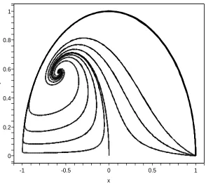
In the following, we will study the simplest model,
¯
β(φ) =mφ2 , V(φ) = 1 2M
0.2
0
x
1 0.5
0 -0.5
-1 y
1
0.8
0.6
0.4
Figure 1: The phase plane of Lorentz violating kinetic dominated solution form >3/8.
wheremandM are parameters. Substituting Eqs. (5.11) into Eqs. (5.2) and (5.3), respec-tively, we obtain
λ1 =λ2=−2√m , Γ1 = Γ2 = 1
2 , (5.12)
and Eqs. (5.6) and (5.7) are trivially satisfied. In the former, Eqs. (5.4) and (5.5) can be fused into the single equation,
x′ =− "
3x− r
3
2(λ1+λ2)
#
(1−x2)
=−3x+ 2√6m(1−x2) , (5.13)
which is one dimensional phase-space corresponding to the unit circle. Critical points cor-respond to fixed points wherex′ = 0, and there are Lorentz violation self-similar solutions
with
H′
H = −3x
2+√6λ
1x . (5.14)
Note that the second term arises from Lorentz violation. Applying the above proce-dure, setting x′ = 0, the critical points (x
0, y0) of the system are (1,0), (−1,0), and (−p
8m/3,p
critical points (1,0) or (−1,0) correspond to two Lorentz violation kinetic-dominated solu-tions. Then, the critical point (−p
8m/3,p1−8m/3) corresponds to a Lorentz violation potential-kinetic solution. Integration of Eq. (5.14) with respect to α will show that all critical points,x0, correspond to the Hubble parameter
H ∝exp
−α
p
. (5.15)
This relates to an expanding universe with a scale factora(t) given bya(t)∼tp, where
0.2
0
x
1 0.5
0 -0.5
-1 y
1
0.8
0.6
0.4
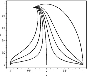
Figure 2: The phase plane of Lorentz violating kinetic-potential solution form <3/8.
p≡ 1
3x2 0−
√
6λ1x0
= 1
3x2 0+ 2
√
6mx0
. (5.16)
The linear perturbation about the points x0+ = +1 and x0− = −1 give the eigenvalues
µ+ = 6 + 4√6m and µ− = 6−4 √
6m, respectively. Thus for positive m, x0+ = +1 is always unstable and x0−=−1 is stable form >3/8 but unstable form <3/8. Moreover,
Another remarkable feature of the above model is that the equation of state is given by
ωφ=−1 + 16
3 m , (5.17)
completely determined by the parameter m of the coupling vector. Thus, we always have
ωφ>−1 for ordinary scalar field.
6. Conclusions
In this paper, we have studied the dynamics of a scalar field in the Lorentz violating scalar-vector-tensor theory of gravity, taking into account the effect of the power-law effective coupling vector. Since the effective coupling vector be dynamics variable, the equation of state is dependent on the coupling parameter. For the model with the power law Hubble parameter and coupling vector, we find an exact solution of the equation of state. A constant equation of state corresponds ton= 2 while forn >2 leads to dynamics equation of states. In this case, the scalar fields are completely associated with the Lorentz violation. Also, the different form in the coupling vector and the potential models lead to the different qualitative evolution in two regimes of inflation. The results show that, for the inverse power-law potential, the Hubble parameter decreases during the Lorentz violation stage and increases in the standard slow roll stage. For the power-law potential, the Hubble parameter increases during the Lorentz violation stage but it decreases in the standard slow roll stage.
From the qualitative study of the dynamical system, we have demonstrated the at-tractor behavior of inflation driven by a scalar field in the context of scalar-vector-tensor theory of gravity. We have found that there exists the Lorentz violating kinetic domi-nated solution and the Lorentz violating potential-kinetic domidomi-nated solution, depending on the region of the coupling parameter in the simplest Lorentz violating chaotic infla-tion model. The quadratic coupling vector and the chaotic potential correspond to the constants λ1 = λ2 = −2√m and Γ1 = Γ2 = 1/2. There are two important results of this study, which are different from the scalar-tensor theory of gravity: the condition for the accelerating universe, Eq. (5.14) and the slope, p, Eq. (5.16). The first one yields
λ1x0 >
p
3/8(ωφ+ 1/3). The analysis of the critical points show that we may obtain an accelerated expansion provided that the solutions are approaching the Lorentz violation kinetic dominated solution withm >1/6 and approaching the Lorentz violation potential-kinetic dominated solution withm <3/8. When the accelerating condition is satisfied, the slope p characterizes the properties of the inflating universe: power-law inflation (p > 0), de Sitter inflation (p= 0) and superinflation (p≡ −|p|<0). In other cases, ifλ1 andλ2are constants, one finds that the coupling vector is still quadratic in scalar field, ¯β ∼φ2, while the potential as a function of scalar fieldφ is given by a power-law potential, V(φ)∼φ2γ
Finally, we would like to emphasize that there exists an attractor solution in the Lorentz violating scalar-vector-tensor theory of gravity.
Acknowledgments
Arianto and Supardi would like to thank BPPS, Dikti, Depdiknas, Republic of Indonesia for financial support. They also wishe to acknowledge all members of Theoretical Physics Laboratory, Faculty of Mathematics and Natural Sciences, ITB, for warmest hospitality. This work is partially supported by Research KK ITB 2007 No. 174/K01.07/PL/07.
References
[1] A. Linde, Particle Physics and Inflationary Cosmology, (Harwood academic publishers, 1980); E. W. Kolb, and M. S. Turner, The Early Universe, (Perseus Publishing, 1990); A. R. Liddle, and D. H. Lyth, Cosmological Inflation and Large-Scale Structure, (Cambridge University Press, Cambridge, 2000).
[2] A Vilenkin, Cosmic Strings and Domain Walls, Phys. Rep.121, 263 (1985); T. W. B. Kibble, Topology of Cosmic Domains and Strings, J. Phys.A9, 1387 (1976); A. Vilenkin and E. P. S. Shellard, Cosmic strings and other topological defects, Cambridge Univ. Press (Cambridge 1994); M. B. Hindmarsh and T. W. Kibble, Cosmic strings, Rept. Prog. Phys.
58, 477 (1995) [arXiv:hep-ph/9411342].
[3] M. B. Green, J. H. Schwarz and E. Witten, Superstring Theory, Vol. 1 and 2, Cambridge Univ. Press (Cambridge 1987).
[4] T. Barreiro, B. de Carlos and E. J. Copeland, Stabilizing the Dilaton in Superstring Cosmology, Phys. Rev. D58, 083513 (1998) [arXiv:hep-th/9805005]; G. Huey, P. J.
Steinhardt, B. A. Ovrut and D. Waldram, A Cosmological Mechanism for Stabilizing Moduli, Phys. Lett. B 476, 379 (2000) [arXiv:hep-th/0001112]; T. Barreiro, B. de Carlos and N. J. Nunes, Moduli Evolution in Heterotic Scenarios, Phys. Lett. B497, 136 (2001)
[arXiv:hep-ph/0010102].
[5] A. Sen,Rolling Tachyon, JHEP0204, 048 (2002) [arXiv:hep-th/0203211]; A. Sen,Tachyon Matter, JHEP0207, 065 (2002) [arXiv:hep-th/0203265].
[6] G. W. Gibbons, Cosmological Evolution of the Rolling Tachyon, Phys. Lett. B537, 1 (2002). [7] A. Sen,Supersymmetric World-volume Action for Non-BPS D-branes, JHEP9910, 008
(1999) [arXiv:hep-th/9909062]; M. Garousi,Tachyon couplings on non-BPS D-branes and Dirac-Born-Infeld action, Nucl. Phys. B 584, 284 (2000) [arXiv:hep-th/0003122]; E. Bergshoeff, M. de Roo, T. de Wit, E. Eyras and S. Panda,T-duality and Actions for
Non-BPS D-branes, JHEP0005, 009 (2000) [arXiv:hep-th/0003221]; J. Kluson,Proposal for non-BPS D-brane action, Phys. Rev. D62, 126003 (2000) [arXiv:hep-th/0004106].
[8] L. Kofman and A. Linde,Problems with Tachyon Inflation, JHEP07, 004 (2002).
[arXiv:hep-th/0205121]; A. Frolov, L. Kofman and A. Starobinsky, Prospects and Problems of Tachyon Matter Cosmology, Phys.Lett. B5458 (2002) [arXiv:hep-th/0204187].
[9] A.G. Riesset al.,Type Ia Supernova Discoveries at z >1 From the Hubble Space Telescope: Evidence for Past Deceleration and Constraints on Dark Energy Evolution, Astrophys. J.
[10] H. Jassal, J. Bagla and T. Padmanabhan,The vanishing phantom menace, [arXiv:astro-ph/0601389].
[11] C. L. Bennettet al., First Year Wilkinson Microwave Anisotropy Probe (WMAP) Observations: Preliminary Maps and Basic Results, Astrophys. J. Suppl.148, 1 (2003) [arXiv:astro-ph/0302207].
[12] C. Wetterich,Cosmology and the fate of dilatation symmetry, Nucl. Phys. B302, 668 (1988); P. J. E. Peebles and B. Ratra,Cosmology with a time-variable cosmological constant,
Astrophys. J. 325, L17 (1988); B. Ratra and P. J. E. Peebles,Cosmological Consequences of a Rolling Homogeneous Scalar Field, Phys. Rev. D37, 3406 (1988); J. A. Frieman,
C. T. Hill, A. Stebbins and I. Waga,Cosmology with Ultra-light Pseudo-Nambu-Goldstone Bosons, Phys. Rev. Lett.75, 2077 (1995) [arXiv:astro-ph/9505060]; R. R. Caldwell, R. Dave and P. J. Steinhardt,Cosmological Imprint of an Energy Component with General Equation of State, Phys. Rev. Lett.80, 1582 (1998) [arXiv:astro-ph/9708069]; I. Zlatev, L. Wang and P. J. Steinhardt,Quintessence, Cosmic Coincidence, and the Cosmological Constant, Phys. Rev. Lett. 82, 896 (1999) [arXiv:astro-ph/9807002].
[13] C. Armendariz-Picon, T. Damour and V. Mukhanov,k-Inflation, Phys. Lett. B458, 209 (1999) [arXiv:hep-th/9904075 ]; C. Armendariz-Picon V. Mukhanov and P.J. Steinhardt,A Dynamical Solution to the Problem of a Small Cosmological Constant and Late-time Cosmic Acceleration, Phys. Rev. Lett. 85, 4438 (2000) [arXiv:astro-ph/0004134]; T. Chiba, T. Okabe and M. Yamaguchi,Kinetically Driven Quintessence, Phys. Rev. D62, 023511 (2000) [arXiv:astro-ph/9912463].
[14] H. Sato,Extremely high energy and violation of Lorentz invariance, [arXiv:astro-ph/0005218]. [15] S. R. Coleman and S. L. Glashow,High-energy tests of Lorentz invariance, Phys. Rev. D59,
116008 (1999) [arXiv:hep-ph/9812418].
[16] S. Kanno and J. Soda,Lorentz violating inflation, Phys. Rev. D74, 063505 (2006) [arXiv:hep-th/0604192].
[17] S. M. Carroll and E. A. Lim,Lorentz-violating vector fields slow the universe down, Phys. Rev. D 70, 123525 (2004) [arXiv:hep-th/0407149].
[18] P. J. Steinhardt L. Wang, and I. Zlatev,Cosmological Tracking Solutions, Phys. Rev. D59, 123504 (1999) [arXiv:astro-ph/9812313].
[19] I. Zlatev and P. J. Steinhardt,A tracker solution to the cold dark matter cosmic coincidence problem, Phys. Lett. B459, 570 (1999) [arXiv:astro-ph/9906481].
[20] J. D. Barrow,Graduated inflationary universe, Phys. Lett. B235, 40 (1990).
[21] P. Binetruy,Models of dynamical supersymmetry breaking and quintessence, Phys. Rev. D60, 063502 (1999) [arXiv:hep-ph/9810553]; P. Brax and J. Martin, The robustness of
quintessence, Phys. Rev. D61, 103502 (2000) [arXiv:astro-ph/9912046].
[22] A. Balbi, C. Baccigalupi, S. Matarrese, F. Perrotta, and N. Vittorio,Implications for
quintessence models from MAXIMA-1 and BOOMERANG-98, Astrophys. J.547, L89 (2001) [arXiv:astro-ph/0009432].