Python Deep Learning Cookbook
Indra den Bakker
Python Deep Learning Cookbook
Copyright © 2017 Packt Publishing
All rights reserved. No part of this book may be reproduced, stored
in a retrieval system, or transmitted in any form or by any means,
without the prior written permission of the publisher, except in the
case of brief quotations embedded in critical articles or reviews.
Every effort has been made in the preparation of this book to
ensure the accuracy of the information presented. However, the
information contained in this book is sold without warranty, either
express or implied. Neither the author, nor Packt Publishing, and its
dealers and distributors will be held liable for any damages caused
or alleged to be caused directly or indirectly by this book.
Packt Publishing has endeavored to provide trademark information
about all of the companies and products mentioned in this book by
the appropriate use of capitals. However, Packt Publishing cannot
guarantee the accuracy of this information.
Published by Packt Publishing Ltd.
Livery Place
35 Livery Street
Birmingham
B3 2PB, UK.
ISBN 978-1-78712-519-3
Credits
Author
Indra den Bakker
Copy Editors
Vikrant Phadkay
Alpha Singh
Reviewer
Radovan Kavicky
Project Coordinator
Commissioning Editor
Veena Pagare
Proofreader
Safis Editing
Acquisition Editor
Vinay Argekar
Indexer
Tejal Daruwale Soni
Content Development Editor
Cheryl Dsa
Graphics
Tania Dutta
Technical Editor
Suwarna Patil
Production Coordinator
About the Author
Indra den Bakker
is an experienced deep learning engineer and
mentor. He is the founder of 23insights—part of NVIDIA's
About the Reviewer
Radovan Kavicky
is the principal data scientist and President at
GapData Institute (
https://www.gapdata.org
) based in Bratislava,
Slovakia, where he harnesses the power of data and the wisdom of
economics for public good.
A macroeconomist by education/academic background and a
consultant and analyst by profession (with more than 8 years of
experience in consulting for clients from the public and private
sector), with strong mathematical and analytical skills, he is able to
deliver top-level research and analytical work. From MATLAB,
SAS, and Stata, he switched to Python, R, and Tableau.
He is a member of the Slovak Economic Association and an
evangelist of open data, open budget initiatives, and open
government partnership. He is the founder of PyData Bratislava, R
<- Slovakia, and SK/CZ Tableau User Group (skczTUG). He has
been a speaker at TechSummit (Bratislava, 2017) and at PyData
(Berlin, 2017), and a member of the global Tableau #DataLeader
network (2017). You can follow him on Twitter at
www.PacktPub.com
For support files and downloads related to your book, please visit
w
ww.PacktPub.com
.
Did you know that Packt offers eBook versions of every book
published, with PDF and ePub files available? You can upgrade to
the eBook version at
www.PacktPub.com
and as a print book
customer, you are entitled to a discount on the eBook copy. Get in
touch with us at
[email protected]for more details.
At
www.PacktPub.com
, you can also read a collection of free
technical articles, sign up for a range of free newsletters and
receive exclusive discounts and offers on Packt books and eBooks.
https://www.packtpub.com/mapt
Get the most in-demand software skills with Mapt. Mapt gives you
full access to all Packt books and video courses, as well as
Why subscribe?
Fully searchable across every book published by Packt
Copy and paste, print, and bookmark content
Customer Feedback
Thanks for purchasing this Packt book. At Packt, quality is at the
heart of our editorial process. To help us improve, please leave us
an honest review on this book's Amazon page at
http://www.amazon.c
om/dp/178712519X
.
If you'd like to join our team of regular reviewers, you can e-mail
us at
[email protected]. We award our regular
reviewers with free eBooks and videos in exchange for their
Table of Contents
Preface
What this book covers
What you need for this book
Who this book is for
Conventions
Reader feedback
Customer support
Downloading the example code
Errata
Piracy
Questions
1.
Programming Environments, GPU Computing, Cloud Solutions, and De
ep Learning Frameworks
Introduction
Setting up a deep learning environment
How to do it...
Launching an instance on Amazon Web Services (AWS)
Getting ready
How to do it...
Launching an instance on Google Cloud Platform (GCP)
Getting ready
How to do it...
Installing CUDA and cuDNN
Getting ready
How to do it...
Installing Anaconda and libraries
How to do it...
Connecting with Jupyter Notebooks on a server
How to do it...
w
How to do it...
Intuitively building networks with Keras
How to do it...
Using PyTorch’s dynamic computation graphs for RNNs
How to do it...
Implementing high-performance models with CNTK
How to do it...
Building efficient models with MXNet
How to do it...
Defining networks using simple and efficient code with Gluon
How to do it...
2.
Feed-Forward Neural Networks
Introduction
Understanding the perceptron
How to do it...
Implementing a single-layer neural network
How to do it...
Building a multi-layer neural network
How to do it...
Getting started with activation functions
How to do it...
Experiment with hidden layers and hidden units
How to do it...
There's more...
Implementing an autoencoder
How to do it...
Tuning the loss function
How to do it...
Experimenting with different optimizers
How to do it...
Adding dropout to prevent overfitting
How to do it...
3.
Convolutional Neural Networks
Introduction
Getting started with filters and parameter sharing
How to do it...
Applying pooling layers
How to do it...
Optimizing with batch normalization
How to do it...
Understanding padding and strides
How to do it...
Experimenting with different types of initialization
How to do it...
Implementing a convolutional autoencoder
How to do it...
Applying a 1D CNN to text
How to do it...
4.
Recurrent Neural Networks
Introduction
Implementing a simple RNN
How to do it...
Adding Long Short-Term Memory (LSTM)
How to do it...
Using gated recurrent units (GRUs)
How to do it...
Implementing bidirectional RNNs
How to do it...
Character-level text generation
How to do it...
5.
Reinforcement Learning
Introduction
Getting ready
How to do it...
Implementing a deep Q-learning algorithm
Getting ready
How to do it...
6.
Generative Adversarial Networks
Introduction
Understanding GANs
How to do it...
Implementing Deep Convolutional GANs (DCGANs)
How to do it...
Upscaling the resolution of images with Super-Resolution GANs (S
RGANs)
How to do it...
7.
Computer Vision
Introduction
Augmenting images with computer vision techniques
How to do it...
Classifying objects in images
How to do it...
Localizing an object in images
How to do it...
Real-time detection frameworks
Segmenting classes in images with U-net
How to do it...
Scene understanding (semantic segmentation)
How to do it...
Finding facial key points
How to do it...
Recognizing faces
How to do it...
8.
Natural Language Processing
9.
Speech Recognition and Video Analysis
Introduction
Implementing a speech recognition pipeline from scratch
How to do it...
Identifying speakers with voice recognition
How to do it...
Understanding videos with deep learning
How to do it...
10.
Time Series and Structured Data
Introduction
Predicting stock prices with neural networks
How to do it...
Predicting bike sharing demand
How to do it...
Using a shallow neural network for binary classification
How to do it...
11.
Game Playing Agents and Robotics
Introduction
Learning to drive a car with end-to-end learning
Getting started
How to do it...
Learning to play games with deep reinforcement learning
How to do it...
12.
Hyperparameter Selection, Tuning, and Neural Network Learning
Introduction
Visualizing training with TensorBoard and Keras
How to do it...
Working with batches and mini-batches
How to do it...
Using grid search for parameter tuning
How to do it...
Learning rates and learning rate schedulers
How to do it...
Comparing optimizers
How to do it...
Determining the depth of the network
Adding dropouts to prevent overfitting
How to do it...
Making a model more robust with data augmentation
How to do it...
Leveraging test-time augmentation (TTA) to boost accuracy
13.
Network Internals
Introduction
Visualizing training with TensorBoard
How to do it..
Visualizing the network architecture with TensorBoard
Analyzing network weights and more
How to do it...
Freezing layers
How to do it...
Storing the network topology and trained weights
How to do it...
14.
Pretrained Models
Introduction
Extracting bottleneck features with ResNet
How to do it...
Leveraging pretrained VGG models for new classes
How to do it...
Preface
Deep learning is revolutionizing a wide range of industries. For
many applications, deep learning has proven to outperform humans
by making faster and more accurate predictions. This book
What this book covers
Chapter 1
,
Programming Environments, GPU Computing, Cloud
Solutions, and Deep Learning Frameworks
, includes information
and recipes related to environments and GPU computing. It is a
must-read for readers who have issues in setting up their
environment on different platforms.
Chapter 2
,
Feed-Forward Neural Networks
, provides a collection of
recipes related to feed-forward neural networks and forms the basis
for the other chapters. The focus of this chapter is to provide
solutions to common implementation problems for different
network topologies.
Chapter 3
,
Convolutional Neural Networks
, focuses on
convolutional neural networks and their application in computer
vision. It provides recipes on techniques and optimizations used in
CNNs.
Chapter 4
,
Recurrent Neural Networks
, provides a collection of
recipes related to recurrent neural networks. These include LSTM
networks and GRUs. The focus of this chapter is to provide
solutions to common implementation problems for recurrent neural
networks.
Chapter 5
,
Reinforcement Learning
, covers recipes for reinforcement
learning with neural networks. The recipes in this chapter introduce
the concepts of deep reinforcement learning in a single-agent
world.
of recipes related to unsupervised learning problems. These include
generative adversarial networks for image generation and super
resolution.
Chapter 7
,
Computer Vision,
contains recipes related to processing
data encoded as images, including video frames. Classic techniques
of processing image data using Python will be provided, along with
best-of-class solutions for detection, classification, and
segmentation.
Chapter 8
,
Natural Language Processing
, contains recipes related to
textual data processing. This includes recipes related to textual
feature representation and processing, including word embeddings
and text data storage.
Chapter 9
,
Speech Recognition and Video Analysis
, covers recipes
related to stream data processing. This includes audio, video, and
frame sequences
Chapter 10
,
Time Series and Structured Data
, provides recipes
related to number crunching. This includes sequences and time
series.
Chapter 11
,
Game Playing Agents and Robotics
, focuses on
state-of-the-art deep learning research applications. This includes recipes
related to game-playing agents in a multi-agent environment
(simulations) and autonomous vehicles.
Chapter 12
,
Hyperparameter Selection, Tuning, and Neural Network
Chapter 13
,
Network Internals
, covers the internals of a neural
network. This includes tensor decomposition, weight initialization,
topology storage, bottleneck features, and corresponding
embedding.
Chapter 14
,
Pretrained Models
, covers popular deep learning models
What you need for this book
Who this book is for
This book is intended for machine learning professionals who are
looking to use deep learning algorithms to create real-world
Conventions
In this book, you will find a number of text styles that distinguish
between different kinds of information. Here are some examples of
these styles and an explanation of their meaning.
Code words in text, database table names, folder names, filenames,
file extensions, pathnames, dummy URLs, user input, and Twitter
handles are shown as follows: "To provide a dummy dataset, we
will use
numpyand the following code."
A block of code is set as follows:
import numpy as np
x_input = np.array([[1,2,3,4,5]]) y_input = np.array([[10]])
Any command-line input or output is written as follows:
curl -O http://developer.download.nvidia.com/compute/cuda/repos/ubuntu1604/x86_64/cuda-repo-ubuntu1604_8.0.61-1_amd64.deb
New terms
and
important words
are shown in bold.
Words that you see on the screen, for example, in menus or dialog
boxes, appear in the text like this:
Warnings or important notes appear like this.
Reader feedback
Feedback from our readers is always welcome. Let us know what
you think about this book-what you liked or disliked. Reader
feedback is important for us as it helps us develop titles that you
will really get the most out of. To send us general feedback, simply
, and mention the book's title in the
Customer support
Downloading the example code
You can download the example code files for this book from your
account at
http://www.packtpub.com
. If you purchased this book
elsewhere, you can visit
http://www.packtpub.com/support
and register
to have the files emailed directly to you. You can download the
code files by following these steps:
1. Log in or register to our website using your email address and
password.
2. Hover the mouse pointer on the SUPPORT tab at the top.
3. Click on Code Downloads & Errata.
4. Enter the name of the book in the Search box.
5. Select the book for which you're looking to download the code
files.
6. Choose from the drop-down menu where you purchased this
book from.
7. Click on Code Download.
Once the file is downloaded, please make sure that you unzip or
extract the folder using the latest version of:
WinRAR / 7-Zip for Windows
Zipeg / iZip / UnRarX for Mac
7-Zip / PeaZip for Linux
The code bundle for the book is also hosted on GitHub at
https://gith
ub.com/PacktPublishing/Python-Deep-Learning-Cookbook
. We also have
Errata
Although we have taken every care to ensure the accuracy of our
content, mistakes do happen. If you find a mistake in one of our
books-maybe a mistake in the text or the code-we would be
grateful if you could report this to us. By doing so, you can save
other readers from frustration and help us improve subsequent
versions of this book. If you find any errata, please report them by
visiting
http://www.packtpub.com/submit-errata
, selecting your book,
clicking on the Errata Submission Form link, and entering the
details of your errata. Once your errata are verified, your
submission will be accepted and the errata will be uploaded to our
website or added to any list of existing errata under the Errata
section of that title. To view the previously submitted errata, go to
https://www.packtpub.com/books/content/support
and enter the name of
Piracy
Piracy of copyrighted material on the internet is an ongoing
problem across all media. At Packt, we take the protection of our
copyright and licenses very seriously. If you come across any
illegal copies of our works in any form on the internet, please
provide us with the location address or website name immediately
so that we can pursue a remedy. Please contact us at
with a link to the suspected pirated
Questions
If you have a problem with any aspect of this book, you can contact
us at
[email protected], and we will do our best to address the
Programming Environments, GPU
Computing, Cloud Solutions, and
Deep Learning Frameworks
This chapter focuses on technical solutions to set up popular deep
learning frameworks. First, we provide solutions to set up a stable
and flexible environment on local machines and with cloud
solutions. Next, all popular Python deep learning frameworks are
discussed in detail:
Setting up a deep learning environment
Launching an instance on Amazon Web Services (AWS)
Launching an instance on Google Cloud Platform (GCP)
Installing CUDA and cuDNN
Installing Anaconda and libraries
Connecting with Jupyter Notebook on a server
Building state-of-the-art, production-ready models with
TensorFlow
Intuitively building networks with Keras
Using PyTorch's dynamic computation graphs for RNNs
Implementing high-performance models with CNTK
Building efficient models with MXNet
Introduction
The recent advancements in deep learning can be, to some extent,
attributed to the advancements in computing power. The increase
in computing power, more specifically the use of GPUs for
processing data, has contributed to the leap from shallow neural
networks to deeper neural networks. In this chapter, we lay the
groundwork for all following chapters by showing you how to set
up stable environments for different deep learning frameworks
used in this cookbook. There are many open source deep learning
frameworks that are used by researchers and in the industry. Each
framework has its own benefits and most of them are supported by
some big tech company.
By following the steps in this first chapter carefully, you should be
able to use local or cloud-based CPUs and GPUs to leverage the
recipes in this book. For this book, we've used Jupyter Notebooks
to execute all code blocks. These notebooks provide interactive
feedback per code block in such a way that it's perfectly suited for
storytelling.
Setting up a deep
learning environment
How to do it...
1. First, you need to check whether you have access to a
CUDA-enabled NVIDIA GPU on your local machine. You can check
the overview at
https://developer.nvidia.com/cuda-gpus
.
2. If your GPU is listed on that page, you can continue installing
CUDA
and
cuDNNif you haven't done that already. Follow the
steps in the
Installing CUDA and cuDNN
section.
Launching an instance on Amazon
Web Services (AWS)
Getting ready
How to do it...
1. Make sure the region you want to work in gives access to P2 or
G3 instances. These instances include
NVIDIA K80
GPUs
and
NVIDIA Tesla M60
GPUs, respectively. The K80 GPU is
faster and has more GPU memory than the M60 GPU: 12 GB
versus 8 GB.
While the NVIDIA K80 and M60 GPUs are powerful
GPUs for running deep learning models, these should
not be considered state-of-the-art. Other faster GPUs
have already been launched by NVIDIA and it takes
some time before these are added to cloud solutions.
However, a big advantage of these cloud machines is
that it is straightforward to scale the number of GPUs
attached to a machine; for example, Amazon's
p2.16xlarge
instance has 16 GPUs.
2. There are two options when launching an AWS instance.
Option 1
: You build everything from scratch.
Option 2
: You
use a preconfigured
Amazon Machine Image
(
AMI
) from
the AWS marketplace. If you choose option 2, you will have to
pay additional costs. For an example, see this AMI at
https://aws
.amazon.com/marketplace/pp/B06VSPXKDX
.
3. Amazon provides a detailed and up-to-date overview of steps
to launch the deep learning AMI at
https://aws.amazon.com/blogs/a
i/get-started-with-deep-learning-using-the-aws-deep-learning-ami/
.
5. Always make sure you stop the running instances when you're
done to prevent unnecessary costs.
A good option to save costs is to use AWS Spot
Launching an instance on Google
Cloud Platform (GCP)
Another popular cloud provider is Google. Its
Google Cloud
Getting ready
How to do it...
1. You need to request an increase in the GPU quota before you
launch a compute instance with a GPU for the first time. Go to
https://console.cloud.google.com/projectselector/iam-admin/quotas
.
2. First, select the project you want to use and apply the Metric
and Region filters accordingly. The GPU instances should
show up as follows:
Figure 1.1: Google Cloud Platform dashboard for increasing the
GPU quotas
3. Select the quota you want to change, click on EDIT QUOTAS,
and follow the steps.
4. You will get an e-mail confirmation when your quota has been
increased.
Installing CUDA and cuDNN
This part is essential if you want to leverage NVIDIA GPUs for
deep learning. The CUDA toolkit is specially designed for
GPU-accelerated applications, where the compiler is optimized for using
math operations. In addition, the
cuDNNlibrary—short for CUDA
Getting ready
Make sure you've registered for
Nvidia's Accelerated Computing
Developer Program
at
https://developer.nvidia.com/cudnn
before
How to do it...
1. We start by downloading NVIDIA with the following
command in the terminal (adjust the download link
accordingly if needed; make sure you use CUDA 8 and not
CUDA 9 for now):
curl -O http://developer.download.nvidia.com/compute/cuda/repos/ubuntu1604/x86_64/cuda-repo-ubuntu1604_8.0.61-1_amd64.deb
2. Next, we unpack the file and update all all packages in the
package lists. Afterwards, we remove the downloaded file:
sudo dpkg -i cuda-repo-ubuntu1604_8.0.61-1_amd64.deb sudo apt-get update
rm cuda-repo-ubuntu1604_8.0.61-1_amd64.deb
3. Now, we're ready to install CUDA with the following
command:
sudo apt-get install cuda-8-0
4. Next, we need to set the environment variables and add them
to the shell script
.bashrc:
echo 'export CUDA_HOME=/usr/local/cuda' >> ~/.bashrc echo 'export PATH=$PATH:$CUDA_HOME/bin' >> ~/.bashrc
echo 'export LD_LIBRARY_PATH=$LD_LIBRARY_PATH:$CUDA_HOME/lib64' >> ~/.bashrc
5. Make sure to reload the shell script afterwards with the
following command:
source ~/.bashrc
correctly installed using the following commands in your
terminal:
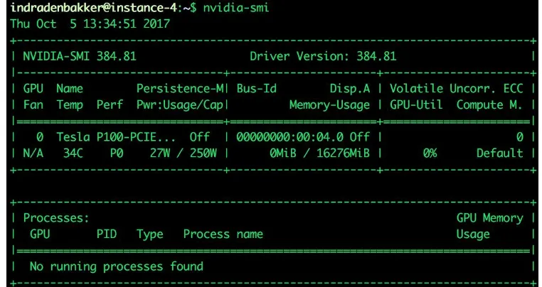
nvcc --version nvidia-smi
The output of the last command should look something like
this:
Figure 1.2: Example output of nvidia-smi showing the connected
GPU
7. Here, we can see that an NVIDIA P100 GPU with 16 GB of
memory is correctly connected and ready to use.
8. We are now ready to install
cuDNN. Make sure the NVIDIA
cuDNNfile is available on the machine, for example, by copying
from your local machine to the server if needed. For Google
cloud compute engine (make sure you've set up
gcloudand the
gcloud compute scp local-directory/cudnn-8.0-linux-x64-v6.0.tgz instance-name
9. First we unpack the file before copying to the right directory as
root:
cd
tar xzvf cudnn-8.0-linux-x64-v6.0.tgz
sudo cp cuda/lib64/* /usr/local/cuda/lib64/
sudo cp cuda/include/cudnn.h /usr/local/cuda/include/
10. To clean up our space, we can remove the files we've used for
installation, as follows:
rm -rf ~/cuda
Installing Anaconda and libraries
How to do it...
1. You can directly download the installation file for Anaconda
on your machine as follows (adjust your Anaconda file
accordingly):
curl -O https://repo.continuum.io/archive/Anaconda3-4.3.1-Linux-x86_64.sh
2. Next, run the bash script (if necessary, adjust the filename
accordingly):
bash Anaconda3-4.3.1-Linux-x86_64.sh
Follow all prompts and choose 'yes' when you're asked to to
add the PATH to the
.bashrcfile (the default is 'no').
3. Afterwards, reload the file:
source ~/.bashrc
4. Now, let's set up an Anaconda environment. Let's start with
copying the files from the GitHub repository and opening the
directory:
git clone https://github.com/indradenbakker/Python-Deep-Learning-Cookbook-Kit.git cd Python-Deep-Learning-Cookbook-Kit
5. Create the environment with the following command:
conda env create -f environment-deep-learning-cookbook.yml
the
.ymlfile. All libraries used in this book are included, for
example, NumPy, OpenCV, Jupyter, and scikit-learn.
7. Activate the environment:
source activate environment-deep-learning-cookbook
Connecting with Jupyter Notebooks
on a server
As mentioned in the introduction, Jupyter Notebooks have gained a
lot of traction in the last couple of years. Notebooks are an intuitive
tool for running blocks of code. When creating the Anaconda
How to do it...
1. If you haven't installed Jupyter yet, you can use the following
command in your activated Anaconda environment on the
server:
conda install jupyter
2. Next, we move back to the terminal on our local machine.
3. One option is to access the Jupyter Notebook running on a
server using SSH-tunnelling. For example, when using Google
Cloud Platform:
gcloud compute ssh --ssh-flag="-L 8888:localhost:8888" --zone "europe-west1-b" "instance-name"
You're now logged in to the server and port
8888on your
local machine will forward to the server with port
8888.
4. Make sure to activate the correct Anaconda environment
before proceeding (adjust the name of your environment
accordingly):
source activate environment-deep-learning-cookbook
5. You can create a dedicated directory for your Jupyter
notebooks:
mkdir notebooks cd notebooks
jupyter notebook
This will start Jupyter Notebook on your server. Next, you can go
to your local browser and access the notebook with the link
provided after starting the notebook, for example,
http://localhost:8888/?
Building state-of-the-art,
production-ready models with
TensorFlow
How to do it...
1. First, we will show how to install TensorFlow from your
terminal (make sure that you adjust the link to the TensorFlow
wheel for your platform and Python version accordingly):
pip install --ignore-installed --upgrade https://storage.googleapis.com/tensorflow/linux/gpu/tensorflow_gpu-1.3.0-cp35-cp35m-linux_x86_64.whl
This will install the GPU-enabled version of TensorFlow
and the correct dependencies.
2. You can now import the TensorFlow library into your Python
environment:
import tensorflow as tf
3. To provide a dummy dataset, we will use
numpyand the
following code:
import numpy as np
x_input = np.array([[1,2,3,4,5]]) y_input = np.array([[10]])
4. When defining a TensorFlow model, you cannot feed the data
directly to your model. You should create a placeholder that
acts like an entry point for your data feed:
x = tf.placeholder(tf.float32, [None, 5]) y = tf.placeholder(tf.float32, [None, 1])
5. Afterwards, you apply some operations to the placeholder with
some variables. For example:
b = tf.Variable(tf.zeros([1])) y_pred = tf.matmul(x, W)+b
6. Next, define a loss function as follows:
loss = tf.reduce_sum(tf.pow((y-y_pred), 2))
7. We need to specify the optimizer and the variable that we want
to minimize:
train = tf.train.GradientDescentOptimizer(0.0001).minimize(loss)
8. In TensorFlow, it's important that you initialize all variables.
Therefore, we create a variable called
init:
init = tf.global_variables_initializer()
We should note that this command doesn't initialize the
variables yet; this is done when we run a session.
9. Next, we create a session and run the training for 10 epochs:
sess = tf.Session() sess.run(init)
for i in range(10):
feed_dict = {x: x_input, y: y_input} sess.run(train, feed_dict=feed_dict)
10. If we also want to extract the costs, we can do so by adding it
as follows:
sess = tf.Session() sess.run(init)
for i in range(10):
feed_dict = {x: x_input, y: y_input}
11. If we want to use multiple GPUs, we should specify this
explicitly. For example, take this part of code from the
TensorFlow documentation:
# Creates a session with log_device_placement set to True.
sess = tf.Session(config=tf.ConfigProto(log_device_placement=True)) # Runs the op.
print(sess.run(sum))
As you can see, this gives a lot of flexibility in how the
computations are handled and by which device.
This is just a brief introduction to how TensorFlow
works. The granular level of model implementation
gives the user a lot of flexibility when implementing
networks. However, if you're new to neural networks, it
might be overwhelming. That is why the Keras
Intuitively building networks with
Keras
Keras is a deep learning framework that is widely known and
adopted by deep learning engineers. It provides a wrapper around
the TensorFlow, CNTK, and the Theano frameworks. This wrapper
you gives the ability to easily create deep learning models by
How to do it...
1. We start by installing Keras on our local Anaconda
environment as follows:
conda install -c conda-forge keras
Make sure your deep learning environment is activated
before executing this command.
2. Next, we import
keraslibrary into our Python environment:
from keras.models import Sequentialfrom keras.layers import Dense
This command outputs the backend used by Keras. By
default, the TensorFlow framework is used:
Figure 1.3: Keras prints the backend used
3. To provide a dummy dataset, we will use
numpyand the
following code:
import numpy as np
x_input = np.array([[1,2,3,4,5]]) y_input = np.array([[10]])
model = Sequential()
model.add(Dense(units=32, input_dim=x_input.shape[1])) model.add(Dense(units=1))
5. Next, we need to compile our model. While compiling, we can
set different settings such as
lossfunction,
optimizer, and
metrics
:
model.compile(loss='mse',
optimizer='sgd',
metrics=['accuracy'])
6. In Keras, you can easily print a summary of your model. It will
also show the number of parameters within the defined model:
model.summary()
In the following figure, you can see the model summary
of our build model:
Figure 1.4: Example of a Keras model summary
7. Training the model is straightforward with one command,
while simultaneously saving the results to a variable called
history
:
8. For testing, the prediction function can be used after training:
pred = model.predict(x_input, batch_size=128)
In this short introduction to Keras, we have
demonstrated how easy it is to implement a neural
network in just a couple of lines of code. However,
don't confuse simplicity with power. The Keras
framework provides much more than we've just
Using PyTorch’s dynamic
computation graphs for RNNs
PyTorch is the Python deep learning framework and it's getting a
lot of traction lately.
PyTorch
is the Python implementation of
Torch, which uses
Lua
.
It is backed by Facebook and is fast thanks
to GPU-accelerated tensor computations. A huge benefit of using
PyTorch over other frameworks is that graphs are created on the fly
and are not static. This means networks are dynamic and you can
adjust your network without having to start over again. As a result,
the graph that is created on the fly can be different for each
How to do it...
1. First, we install PyTorch in our Anaconda environment, as
follows:
conda install pytorch torchvision cuda80 -c soumith
If you want to install PyTorch on another platform, you
can have a look at the PyTorch website for clear
guidance:
http://pytorch.org/
.
2. Let's import PyTorch into our Python environment:
import torch
3. While Keras provides higher-level abstraction for building
neural networks, PyTorch has this feature built in. This means
one can build with higher-level building blocks or can even
build the forward and backward pass manually. In this
introduction, we will use the higher-level abstraction. First, we
need to set the size of our random training data:
batch_size = 32 input_shape = 5 output_shape = 10
4. To make use of GPUs, we will cast the tensors as follows:
torch.set_default_tensor_type('torch.cuda.FloatTensor')
5. We can use this to generate random training data:
from torch.autograd import Variable
X = Variable(torch.randn(batch_size, input_shape))
y = Variable(torch.randn(batch_size, output_shape), requires_grad=False)
6. We will use a simple neural network having one hidden layer
with 32 units and an output layer:
model = torch.nn.Sequential(
torch.nn.Linear(input_shape, 32), torch.nn.Linear(32, output_shape), ).cuda()
We use the
.cuda()extension to make sure the model
runs on the GPU.
7. Next, we define the MSE loss function:
loss_function = torch.nn.MSELoss()
8. We are now ready to start training our model for 10 epochs
with the following code:
learning_rate = 0.001 for i in range(10): y_pred = model(x)
loss = loss_function(y_pred, y) print(loss.data[0])
# Zero gradients model.zero_grad() loss.backward()
# Update weights
for param in model.parameters():
param.data -= learning_rate * param.grad.data
deep learning models. What we didn't demonstrate in
this introduction, is the use of dynamic graphs in
Implementing high-performance
models with CNTK
How to do it...
1. First, we install
CNTKwith
pipas follows:
pip install https://cntk.ai/PythonWheel/GPU/cntk-2.2-cp35-cp35m-linux_x86_64.whl
Adjust the wheel file if necessary (see
https://docs.microsoft
.com/en-us/cognitive-toolkit/Setup-Linux-Python?
tabs=cntkpy22
).
2. After installing CNTK, we can import it into our Python
environment:
import cntk
3. Let's create some simple dummy data that we can use for
training:
import numpy as np
x_input = np.array([[1,2,3,4,5]], np.float32) y_input = np.array([[10]], np.float32)
4. Next, we need to define the placeholders for the input data:
X = cntk.input_variable(5, np.float32) y = cntk.input_variable(1, np.float32)
5. With CNTK, it's straightforward to stack multiple layers. We
stack a dense layer with 32 inputs on top of an output layer
with 1 output:
from cntk.layers import Dense, Sequential model = Sequential([Dense(32),
6. Next, we define the loss function:
loss = cntk.squared_error(model, y)
7. Now, we are ready to finalize our model with an optimizer:
learning_rate = 0.001
trainer = cntk.Trainer(model, (loss), cntk.adagrad(model.parameters, learning_rate))
8. Finally, we can train our model as follows:
for epoch in range(10):
trainer.train_minibatch({X: x_input, y: y_input})
Building efficient models with
MXNet
The MXNet deep learning framework allows you to build efficient
deep learning models in Python. Next to Python, it also let you
build models in popular languages as R, Scala, and Julia. Apache
MXNet is supported by Amazon and Baidu, amongst others.
MXNet has proven to be fast in benchmarks and it supports GPU
and multi-GPU usages. By using lazy evaluation, MXNet is able to
automatically execute operations in parallel. Furthermore, the
How to do it...
1. To install MXNet on Ubuntu with GPU support, we can use
the following command in the terminal:
pip install mxnet-cu80==0.11.0
For other platforms and non-GPU support, have a look at
https://mxnet.incubator.apache.org/get_started/install.html
.
2. Next, we are ready to import
mxnetin our Python environment:
import mxnet as mx3. We create some simple dummy data that we assign to the GPU
and CPU:
import numpy as np
x_input = mx.nd.empty((1, 5), mx.gpu())
x_input[:] = np.array([[1,2,3,4,5]], np.float32)
y_input = mx.nd.empty((1, 5), mx.cpu())
y_input[:] = np.array([[10, 15, 20, 22.5, 25]], np.float32)
4. We can easily copy and adjust the data. Where possible
MXNet will automatically execute operations in parallel:
x_input
w_input = x_input
z_input = x_input.copyto(mx.cpu()) x_input += 1
w_input /= 2 z_input *= 2
print(x_input.asnumpy())
train_iter = mx.io.NDArrayIter(x_input, y_input, batch_size, shuffle=True, data_name='input', label_name='target')
7. Next, we can create the symbols for our model:
X = mx.sym.Variable('input') Y = mx.symbol.Variable('target')
fc1 = mx.sym.FullyConnected(data=X, name='fc1', num_hidden = 5)
lin_reg = mx.sym.LinearRegressionOutput(data=fc1, label=Y, name="lin_reg")
8. Before we can start training, we need to define our model:
model = mx.mod.Module( symbol = lin_reg,
data_names=['input'], label_names = ['target'] )
9. Let's start training:
model.fit(train_iter,
optimizer_params={'learning_rate':0.01, 'momentum': 0.9}, num_epoch=100,
batch_end_callback = mx.callback.Speedometer(batch_size, 2))
10. To use the trained model for prediction we:
model.predict(train_iter).asnumpy()
Defining networks using simple and
efficient code with Gluon
The newest addition to the broad range of deep learning
frameworks is Gluon. Gluon is recently launched by AWS and
Microsoft to provide an API with simple, easy-to-understand code
without the loss of performance. Gluon is already included in the
latest release of MXNet and will be available in future releases of
CNTK (and other frameworks). Just like Keras, Gluon is a wrapper
around other deep learning frameworks. The main difference
How to do it...
1. At the moment,
gluonis included in the latest release of
MXNet (follow the steps in
Building efficient models with
MXNet
to install MXNet).
2. After installing, we can directly import
gluonas follows:
from mxnet import gluon3. Next, we create some dummy data. For this we need the data to
be in MXNet's NDArray or Symbol:
import mxnet as mx import numpy as np
x_input = mx.nd.empty((1, 5), mx.gpu())
x_input[:] = np.array([[1,2,3,4,5]], np.float32)
y_input = mx.nd.empty((1, 5), mx.gpu())
y_input[:] = np.array([[10, 15, 20, 22.5, 25]], np.float32)
4. With Gluon, it's really straightforward to build a neural
network by stacking layers:
net = gluon.nn.Sequential() with net.name_scope():
net.add(gluon.nn.Dense(16, activation="relu")) net.add(gluon.nn.Dense(len(y_input)))
5. Next, we initialize the parameters and we store these on our
GPU as follows:
net.collect_params().initialize(mx.init.Normal(), ctx=mx.gpu())
softmax_cross_entropy = gluon.loss.SoftmaxCrossEntropyLoss()
trainer = gluon.Trainer(net.collect_params(), 'adam', {'learning_rate': .1})
7. We're ready to start training or model:
n_epochs = 10
for e in range(n_epochs):
for i in range(len(x_input)): input = x_input[i]
target = y_input[i]
with mx.autograd.record(): output = net(input)
loss = softmax_cross_entropy(output, target) loss.backward()
trainer.step(input.shape[0])
Feed-Forward Neural Networks
In this chapter, we will implement
Feed-Forward Neural
Networks
(
FNN
) and discuss the building blocks for deep
learning:
Understanding the perceptron
Implementing a single-layer neural network
Building a multi-layer neural network
Getting started with activation functions
Hidden layers and hidden units
Implementing an autoencoder
Tuning the loss function
Introduction
The focus of this chapter is to provide solutions to common
implementation problems for FNN and other network topologies.
The techniques discussed in this chapter also apply to the
following chapters.
FNNs are networks where the information only moves in one
direction and does not cycle (as we will see in
Chapter 4
,
Recurrent
Neural Networks
). FNNs are mainly used for supervised learning
where the data is not sequential or time-dependent, for example for
general classification and regression tasks. We will start by
introducing a perceptron and we will show how to implement a
perceptron with NumPy. A perceptron demonstrates the mechanics
of a single unit. Next, we will increase the complexity by
increasing the number of units and introduce single-layer and
multi-layer neural networks. The high number of units, in
Understanding the perceptron
First, we need to understand the basics of neural networks. A
neural network consists of one or multiple layers of
neurons
,
named after the biological neurons in human brains. We
will demonstrate the mechanics of a single neuron by implementing
a perceptron. In a perceptron, a single unit (neuron) performs all
the computations. Later, we will scale the number of units to create
deep neural networks:
Figure 2.1: Perceptron
A perceptron can have multiple inputs. On these inputs, the unit
performs some computations and outputs a single value, for
These computations can easily be scaled to high dimensional input.
An
activation function
(
φ
) determines the final output of the
perceptron in the
forward pass
:
The weights and bias are randomly initialized. After each
epoch
(iteration over the training data), the weights are updated based on
the difference between the output and the desired output (
error
)
multiplied by the
learning rate
. As a consequence, the weights
will be updated towards the training data (
backward pass
) and the
accuracy of the output will improve. Basically, the perceptron is a
linear combination optimized on the training data. As an activation
function we will use a unit step function: if the output is above a
certain threshold the output will be activated (hence a 0 versus 1
binary classifier). A perceptron is able to classify classes with
100% accuracy if the classes are linearly separable. In the next
recipe, we will show you how to implement a perceptron
How to do it...
1. Import the libraries and dataset as follows:
import numpy as np
from sklearn.model_selection import train_test_split import matplotlib.pyplot as plt
# We will be using the Iris Plants Database from sklearn.datasets import load_iris
SEED = 2017
2. First, we subset the imported data as shown here:
# The first two classes (Iris-Setosa and Iris-Versicolour) are linear separable iris = load_iris()
idxs = np.where(iris.target<2) X = iris.data[idxs]
y = iris.target[idxs]
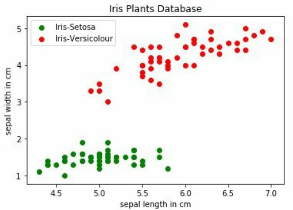
3. Let's plot the data for two of the four variables with the
following code snippet:
plt.scatter(X[Y==0][:,0],X[Y==0][:,2], color='green', label='Iris-Setosa') plt.scatter(X[Y==1][:,0],X[Y==1][:,2], color='red', label='Iris-Versicolour') plt.title('Iris Plants Database')
plt.xlabel('sepal length in cm') plt.ylabel('sepal width in cm') plt.legend()
plt.show()
Figure 2.2: Iris plants database (two classes)
4. To validate our results, we split the data into training and
validation sets as follows:
X_train, X_val, y_train, y_val = train_test_split(X, y, test_size=0.2, random_state=SEED)
5. Next, we initialize the
weightsand the
biasfor the perceptron:
weights = np.random.normal(size=X_train.shape[1])bias = 1
6. Before training, we need to define the hyperparameters:
learning_rate = 0.1 n_epochs = 15
7. Now, we can start training our perceptron with a
forloop:
del_w = np.zeros(weights.shape)hist_loss = [] hist_accuracy = []
for i in range(n_epochs):
output = np.where((X_train.dot(weights)+bias)>0.5, 1, 0)
# Compute MSE
error = np.mean((y_train-output)**2)
# Update weights and bias
weights-= learning_rate * np.dot((output-y_train), X_train)
bias += learning_rate * np.sum(np.dot((output-y_train), X_train))
# Calculate MSE
loss = np.mean((output - y_train) ** 2) hist_loss.append(loss)
# Determine validation accuracy
output_val = np.where(X_val.dot(weights)>0.5, 1, 0) accuracy = np.mean(np.where(y_val==output_val, 1, 0)) hist_accuracy.append(accuracy)
8. We've saved the training loss and validation accuracy so that
we can plot them:
fig = plt.figure(figsize=(8, 4)) a = fig.add_subplot(1,2,1)
Implementing a single-layer neural
network
Now we can move on to
neural networks
. We will start by
implementing the simplest form of a neural network: a single-layer
neural network. The difference from a perceptron is that the
computations are done by multiple units (neurons), hence a
network. As you may expect, adding more units will increase the
number of problems that can be solved. The units perform their
computations separately and are stacked in a layer; we call this
layer the
hidden layer
. Therefore, we call the units stacked in this
layer the
hidden units
. For now, we will only consider a single
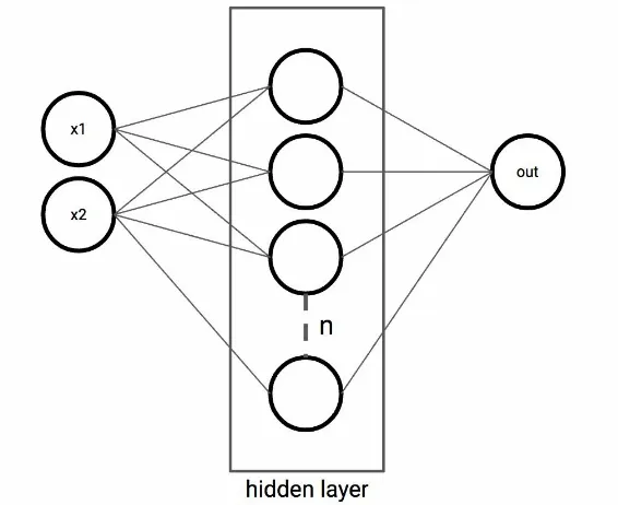
hidden layer. The output layer performs as a perceptron. This time,
as input we have the hidden units in the hidden layer instead of the
input variables:
variables,
n
hidden units, and a single output unit
In our implementation of the perceptron, we've used a unit
step function to determine the class. In the next recipe, we will use
a non-linear activation function sigmoid for the hidden units and
the output function. By replacing the step function with a
linear activation function, the network will be able to uncover
non-linear patterns as well. More on this later in the
Activation
functions
section. In the backward pass, we use the derivative of
the sigmoid to update the weights.
How to do it...
1. Import libraries and dataset:
import numpy as np
from sklearn.model_selection import train_test_split import matplotlib.pyplot as plt
# We will be using make_circles from scikit-learn from sklearn.datasets import make_circles
SEED = 2017
2. First, we need to create the training data:
# We create an inner and outer circle
X, y = make_circles(n_samples=400, factor=.3, noise=.05, random_state=2017) outer = y == 0
inner = y == 1
3. Let's plot the data to show the two classes:
plt.title("Two Circles")
Figure 2.5: Example of non-linearly separable data
4. We normalize the data to make sure the center of both circles
is
(1,1)
:
X = X+1
5. To determine the performance of our algorithm we split our
data:
X_train, X_val, y_train, y_val = train_test_split(X, y, test_size=0.2, random_state=SEED)
6. A linear activation function won't work in this case, so we'll be
using a
sigmoidfunction:
def sigmoid(x):
return 1 / (1 + np.exp(-x))
7. Next, we define the hyperparameters:
n_hidden = 50 # number of hidden units n_epochs = 1000
learning_rate = 1
8. Initialize the weights and other variables:
# Initialise weights
weights_hidden = np.random.normal(0.0, size=(X_train.shape[1], n_hidden)) weights_output = np.random.normal(0.0, size=(n_hidden))
hist_loss = [] hist_accuracy = []
9. Run the single-layer neural network and output the statistics:
for e in range(n_epochs):
# Loop through training data in batches of 1 for x_, y_ in zip(X_train, y_train):
# Forward computations
hidden_input = np.dot(x_, weights_hidden) hidden_output = sigmoid(hidden_input)
output = sigmoid(np.dot(hidden_output, weights_output))
# Backward computations error = y_ - output
output_error = error * output * (1 - output)
hidden_error = np.dot(output_error, weights_output) * hidden_output * (1 - hidden_output)
del_w_output += output_error * hidden_output del_w_hidden += hidden_error * x_[:, None]
# Update weights
weights_hidden += learning_rate * del_w_hidden / X_train.shape[0] weights_output += learning_rate * del_w_output / X_train.shape[0]
# Print stats (validation loss and accuracy) if e % 100 == 0:
hidden_output = sigmoid(np.dot(X_val, weights_hidden)) out = sigmoid(np.dot(hidden_output, weights_output)) loss = np.mean((out - y_val) ** 2)
# Final prediction is based on a threshold of 0.5 predictions = out > 0.5
accuracy = np.mean(predictions == y_val) print("Epoch: ", '{:>4}'.format(e),
"; Validation loss: ", '{:>6}'.format(loss.round(4)),
"; Validation accuracy: ", '{:>6}'.format(accuracy.round(4)))
Building a multi-layer neural
network
What we've created in the previous recipe is actually the simplest
form of an FNN: a neural network where the information flows
only in one direction. For our next recipe, we will extend the
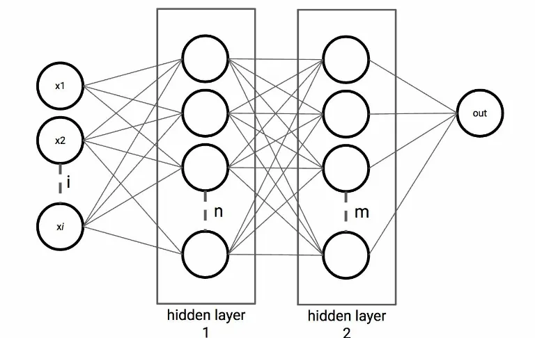
number of hidden layers from one to multiple layers. Adding
additional layers increases the power of a network to learn complex
non-linear patterns.
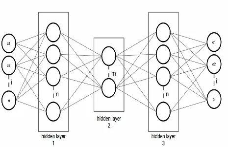
Figure 2.7: Two-layer neural network with
i
input variables,
n
hidden units, and
m
hidden units respectively, and a single output
unit
increases exponentially. In the next recipe, we will create a
network with two hidden layers to predict wine quality. This is a
regression task, so we will be using a linear activation for the
output layer. For the hidden layers, we use ReLU activation
How to do it...
1. We start by import the libraries as follows:
import numpy as np import pandas as pd
from sklearn.model_selection import train_test_split
from keras.models import Sequential from keras.layers import Dense
from keras.callbacks import EarlyStopping, ModelCheckpoint from keras.optimizers import Adam
from sklearn.preprocessing import StandardScaler
SEED = 2017
2. Load dataset:
data = pd.read_csv('Data/winequality-red.csv', sep=';') y = data['quality']
X = data.drop(['quality'], axis=1)
3. Split data for training and testing:
X_train, X_test, y_train, y_test = train_test_split(X, y, test_size=0.2, random_state=SEED)
4. Print average quality and first rows of training set:
print('Average quality training set: {:.4f}'.format(y_train.mean())) X_train.head()
Figure 2-8: Training data
5. An important next step is to normalize the input data:
scaler = StandardScaler().fit(X_train)
X_train = pd.DataFrame(scaler.transform(X_train)) X_test = pd.DataFrame(scaler.transform(X_test))
6. Determine baseline predictions:
# Predict the mean quality of the training data for each validation input
print('MSE:', np.mean((y_test - ([y_train.mean()] * y_test.shape[0])) ** 2).round(4)) ## MSE: 0.594
7. Now, let's build our neural network by defining the network
architecture:
model = Sequential()
# First hidden layer with 100 hidden units
model.add(Dense(200, input_dim=X_train.shape[1], activation='relu')) # Second hidden layer with 50 hidden units
model.add(Dense(25, activation='relu')) # Output layer
model.add(Dense(1, activation='linear')) # Set optimizer
opt = Adam() # Compile model
model.compile(loss='mse', optimizer=opt, metrics=['accuracy'])
callbacks = [
EarlyStopping(monitor='val_acc', patience=20, verbose=2),
ModelCheckpoint('checkpoints/multi_layer_best_model.h5', monitor='val_acc', save_best_only=True, verbose=0) ]
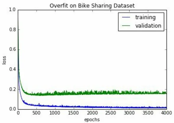
9. Run the model with a batch size of 64, 5,000 epochs, and a
validation split of 20%:
batch_size = 64 n_epochs = 5000
model.fit(X_train.values, y_train, batch_size=batch_size, epochs=n_epochs, validation_split=0.2, verbose=2,
callbacks=callbacks)
10. We can now print the performance on the test set after loading
the optimal weights:
best_model = model
best_model.load_weights('checkpoints/multi_layer_best_model.h5')
best_model.compile(loss='mse', optimizer='adam', metrics=['accuracy'])
# Evaluate on test set
score = best_model.evaluate(X_test.values, y_test, verbose=0) print('Test accuracy: %.2f%%' % (score[1]*100))
## Test accuracy: 66.25%
## Benchmark accuracy on dataset 62.4%
Getting started with activation
functions
If we only use linear activation functions, a neural network would
represent a large collection of linear combinations. However, the
power of neural networks lies in their ability to model complex
nonlinear behavior. We briefly introduced the non-linear activation
functions sigmoid and ReLU in the previous recipes, and there are
many more popular nonlinear activation functions, such as
ELU
,
Leaky ReLU
,
TanH
, and
Maxout
.
There is no general rule as to which activation works best for the
hidden units. Deep learning is a relatively new field and most
results are obtained by trial and error instead of mathematical
proofs. For the output unit, we use a single output unit and a linear
activation function for regression tasks. For classification tasks
with n classes, we use
n
output nodes and a softmax activation
function. The softmax function forces the network to output
probabilities between
0
and
1
for mutually exclusive classes and
the probabilities sum up to
1
. For binary classification, we can also
use a single output node and a sigmoid activation function to output
probabilities.
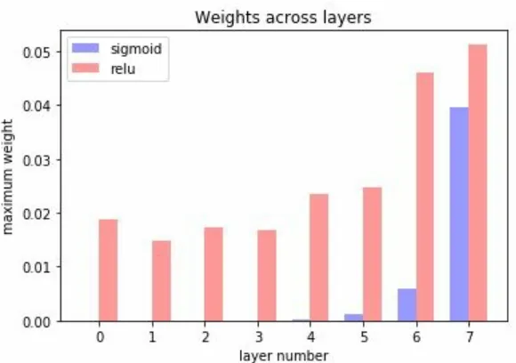
problem). This holds especially when activation functions have a
derivative that only takes on small values (for example the sigmoid
activation function) or activation functions that have a derivative
that can take values that are larger than
1
.
Activation functions such as the ReLU prevents such cases.
The ReLU has a derivative of
1
when the output is positive and is
0
How to do it...
1. Import the libraries as follows:
import numpy as np import pandas as pd
from sklearn.model_selection import train_test_split import matplotlib.pyplot as plt
from keras.models import Sequential from keras.layers import Dense
from keras.utils import to_categorical from keras.callbacks import Callback
from keras.datasets import mnist
SEED = 2017
2. Load the MNIST dataset:
(X_train, y_train), (X_val, y_val) = mnist.load_data()
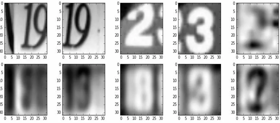
3. Show an example of each label and print the count per label:
# Plot first image of each label unique_labels = set(y_train) plt.figure(figsize=(12, 12))
i = 1
for label in unique_labels:
image = X_train[y_train.tolist().index(label)] plt.subplot(10, 10, i)
plt.axis('off')
plt.title("{0}: ({1})".format(label, y_train.tolist().count(label))) i += 1
_ = plt.imshow(image, cmap='gray') plt.show()
Figure 2.9: Examples of labels (and count) in the MNIST dataset
4. Preprocess the data:
# Normalize data
X_train = X_train.astype('float32')/255. X_val = X_val.astype('float32')/255.
# One-Hot-Encode labels
y_train = np_utils.to_categorical(y_train, 10) y_val = np_utils.to_categorical(y_val, 10)
# Flatten data - we threat the image as a sequential array of values X_train = np.reshape(X_train, (60000, 784))
X_val = np.reshape(X_val, (10000, 784))
5. Define the model with the sigmoid activation function:
model_sigmoid = Sequential()
# Compile model with SGD
model_sigmoid.compile(loss='categorical_crossentropy', optimizer='sgd', metrics=['accuracy'])
6. Define the model with the ReLU activation function:
model_relu = Sequential()
model_relu.add(Dense(700, input_dim=784, activation='relu')) model_relu.add(Dense(700, activation='relu'))