Data Deduplication for Data Optimization for Storage and Network Systems pdf pdf

(1)

Daehee Kim

Sejun Song

Baek-Young Choi

Data

Deduplication for

Data Optimization

for Storage and

(2)

(3)

(4)

Optimization for Storage

and Network Systems

(5)

Daehee Kim

Department of Computing and New Media Technologies University of Wisconsin-Stevens Point Stevens Point, Wisconsin, USA

Baek-Young Choi

Department of Computer Science and Electrical Engineering University of Missouri-Kansas City Kansas City, Missouri, USA

Sejun Song

Department of Computer Science and Electrical Engineering University of Missouri-Kansas City Kansas City, Missouri, USA

ISBN 978-3-319-42278-7 ISBN 978-3-319-42280-0 (eBook) DOI 10.1007/978-3-319-42280-0

Library of Congress Control Number: 2016949407

This work is subject to copyright. All rights are reserved by the Publisher, whether the whole or part of the material is concerned, specifically the rights of translation, reprinting, reuse of illustrations, recitation, broadcasting, reproduction on microfilms or in any other physical way, and transmission or information storage and retrieval, electronic adaptation, computer software, or by similar or dissimilar methodology now known or hereafter developed.

The use of general descriptive names, registered names, trademarks, service marks, etc. in this publication does not imply, even in the absence of a specific statement, that such names are exempt from the relevant protective laws and regulations and therefore free for general use.

The publisher, the authors and the editors are safe to assume that the advice and information in this book are believed to be true and accurate at the date of publication. Neither the publisher nor the authors or the editors give a warranty, express or implied, with respect to the material contained herein or for any errors or omissions that may have been made.

Printed on acid-free paper

This Springer imprint is published by Springer Nature

(6)

Part I Traditional Deduplication Techniques and Solutions

1 Introduction . . . 3

1.1 Data Explosion. . . 3

1.2 Redundancies. . . 4

1.3 Existing Deduplication Solutions to Remove Redundancies. . . 5

1.4 Issues Related to Existing Solutions. . . 7

1.5 Deduplication Framework. . . 7

1.6 Redundant Array of Inexpensive Disks. . . 8

1.7 Direct-Attached Storage. . . 9

1.8 Storage Area Network. . . 10

1.9 Network-Attached Storage. . . 12

1.10 Comparison of DAS, NAS and SAN . . . 13

1.11 Storage Virtualization . . . 13

1.12 In-Memory Storage. . . 15

1.13 Object-Oriented Storage. . . 16

1.14 Standards and Efforts to Develop Data Storage Systems. . . 16

1.15 Summary and Organization. . . 20

References. . . 21

2 Existing Deduplication Techniques . . . 23

2.1 Deduplication Techniques Classification. . . 23

2.2 Common Modules. . . 25

2.2.1 Chunk Index Cache . . . 25

2.2.2 Bloom Filter. . . 30

2.3 Deduplication Techniques by Granularity. . . 34

2.3.1 File-Level Deduplication. . . 34

2.3.2 Fixed-Size Block Deduplication. . . 38

2.3.3 Variable-Sized Block Deduplication . . . 44

2.3.4 Hybrid Deduplication. . . 54

2.3.5 Object-Level Deduplication. . . 55

2.3.6 Comparison of Deduplications by Granularity. . . 55

(7)

vi Contents

(8)

5.2 Software-Defined Network. . . 121

5.3 Control and Data Flow . . . 121

5.4 Encoding Algorithms in Middlebox (SDMB). . . 124

5.5 Index Distribution Algorithms. . . 125

5.5.1 SoftDANCE-Full (SD-Full). . . 125

5.5.2 SoftDance-Uniform (SD-Uniform). . . 126

5.5.3 SoftDANCE-Merge (SD-Merge). . . 127

5.5.4 SoftDANCE-Optimize (SD-opt). . . 128

5.6 Implementation. . . 130

5.6.1 Floodlight, REST, JSON. . . 130

5.6.2 CPLEX Optimizer: Installation. . . 130

5.6.3 CPLEX Optimizer: Run Simple CPLEX Using Interactive Optimizer. . . 135

5.6.4 CPLEX Optimizer: Run Simple CPLEX Using Java Application (with CPLEX API). . . 137

5.7 Setup . . . 139

5.7.1 Experiment. . . 139

5.7.2 Emulation. . . 140

5.8 Evaluation. . . 140

5.8.1 Metrics. . . 140

5.8.2 Data Sets. . . 142

5.8.3 Storage Space and Network Bandwidth Saving . . . 142

5.8.4 CPU and Memory Overhead. . . 143

5.8.5 Performance and Overhead per Topology. . . 145

5.8.6 SoftDance vs. Combined Existing Deduplication Techniques. . . 147

5.9 Summary. . . 150

References. . . 151

Part IV Future Directions 6 Mobile De-Duplication. . . 155

6.1 Large Redundancies in Mobile Devices. . . 155

6.2 Approaches and Observations. . . 156

6.3 JPEG and MPEG4. . . 156

6.4 Evaluation. . . 156

(9)

viii Contents

6.4.2 Throughput and Running Time per File Type. . . 158

6.4.3 Throughput and Running Time per File Size. . . 161

6.5 Summary. . . 161

References. . . 164

7 Conclusions. . . 165

Part V Appendixes Appendices. . . 169

A Index Creation with SHA1. . . 171

A.1 sha1Wrapper.h. . . 171

A.2 sha1Wrapper.cc. . . 172

A.3 sha1.h. . . 173

A.4 sha1.cc. . . 177

B Index Table Implementation using Unordered Map. . . 193

B.1 cacheInterface.h. . . 193

B.2 cache.h . . . 195

B.3 cache.cc. . . 198

C Bloom Filter Implementation. . . 201

C.1 bf.h. . . 201

C.2 bf.c. . . 202

D Rabin Fingerprinting Implementation. . . 209

D.1 rabinpoly.h . . . 209

D.2 rabinpoly.cc. . . 211

D.3 rabinpoly_main.cc. . . 216

E Chunking Core Implementation . . . 219

E.1 chunk.h. . . 219

E.2 chunk_main.cc. . . 221

E.3 chunk_sub.cc. . . 223

E.4 common.h. . . 226

E.5 util.cc. . . 227

F Chunking Wrapper Implementation. . . 231

F.1 chunkInterface.h. . . 231

F.2 chunkWrapper.h . . . 233

F.3 chunkWrapper.cc. . . 233

(10)

(11)

(12)

ACK Acknowledgement AES_NI AES New Instruction

AES Advanced Encryption Standard AFS Andrew File System

CAS Content address storage CDB Command descriptor block CDMI Cloud Data Management Interface CDN Content Delivery Network

CDNI Content delivery network interconnection CIFS Common Internet File System

CRC Cyclic redundancy check CSP Content service provider DAS Direct-attached storage dCDN downstream CDN DCN Data centre network

DCT Discrete cosine transformation DDFS Data Domain File System DES Data Encryption Standard DHT Distributed hash table

EDA Email deduplication algorithm EMC EMC Corporation

FC Fibre channel

FIPS Federal Information Processing Standard FUSE File System in UserSpace

HEDS Hybrid email deduplication system ICN Information-centric networking IDC International Data Corporation IDE Integrated development environment iFCP Internet Fibre Channel Protocol I-frame Intra frame

IP Internet Protocol

(13)

xii Acronyms

ONC RPC Open Networking Computing Remote Procedure Call PATA Parallel ATA

SAFE Structure-Aware File and Email Deduplication for Cloud-based Storage Systems

SoftDance Software-defined deduplication as a network and storage service SSHD Solid-state hybrid drive

SSL Secure Socket Layer

(14)

(15)

Part I

Traditional Deduplication Techniques

and Solutions

In this part, we present an overview of data deduplication. In Chap.1, we show the importance of data deduplication by pointing out data explosion and large amounts of redundancies. We describe design and issues in connection with current solutions, including storage data deduplication, redundancy elimination, and information-centric networking. We introduce a deduplication framework that optimizes data from clients to servers through networks. The framework consists of three components based on the level of deduplication: the client component removes local redundancies that occur in a client, the network component removes redundant transfers coming from different clients using redundancy elimination (RE) devices, and the server component eliminates redundancies coming from different networks. We also present the evolution of data storage systems. Data storage systems evolved from storage devices attached to a single computer (direct-attached storage) into storage devices attached to computer networks (storage area network and network-attached storage). We discuss the different kinds of storage being developed and how they differ from one another. We explain the concepts redundant array of inexpensive disks (RAID), direct-attached storage (DAS), storage area network (SAN), and network-attached storage (NAS). A storage virtualization technique known as software-defined storage is discussed.

(16)

data explosion and large amounts of redundancies. We elaborate on current solutions (including storage data deduplication, redundancy elimination, information-centric networking) for data deduplication and the limitations of current solutions. We introduce a deduplication framework that optimizes data from clients to servers through networks. The framework consists of three components based on the level of deduplication. The client component removes local redundancies that occur in a client, the network component removes redundant transfers coming from different clients using redundancy elimination (RE) devices, and the server component elimi-nates redundancies coming from different networks. Then we show the evolution of data storage. Data storage has evolved from storage devices attached to a single computer (direct-attached storage) into storage devices attached to computer networks (storage area network and network-attached storage). We discuss the different kinds of storage devices and how they differ from one another. A redundant array of inexpensive disks (RAID), which improves storage access performance, is explained, and direct-attached storage (DAS), where storage is incorporated into a computer, is illustrated. We elaborate on storage area networks (SANs) and network-attached storage (NAS), where data from computers are transferred to storage devices through a dedicated network (SAN) or a general local area network used for sending and receiving application data (NAS). SAN and NAS consolidate and efficiently provide storage without wasting storage space compared to a DAS device. We describe a storage virtualization technique known as software-defined storage.

1.1 Data Explosion

We live in an era of data explosion. Based on the International Data Corporation’s (IDC’s) Digital Universe Study [6] , as shown in Fig.1.1, data volume will increase by 50 times by the end of 2020 over its 2010 level; this amounts to 40 zetabytes (40 million petabytes – more than 5200 gigabytes for every person). This huge increase in data volume will have a critical impact on the overhead costs of

D. Kim et al.,Data Deduplication for Data Optimization for Storage and Network Systems, DOI 10.1007/978-3-319-42280-0_1

(17)

4 1 Introduction

Fig. 1.1 Data explosion: IDC’s Digital Universe Study [6]

computation, storage and networks. Also, large portions of the data will contain massive redundancies created by users, applications, systems and communication models.

Interestingly, massive portions of this enormous amount of data will be derived from redundancies in storage devices and networks. One study [9] showed that there is a redundancy of 70 % in data sets collected from file systems of almost 1000 computers in an enterprise. Another study [17] found that 30 % of incoming traffic and 60 % of outgoing traffic are redundant based on packet traces on a corporate research environment with 3000 users and Web servers.

1.2 Redundancies

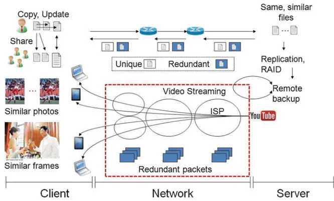
Redundancies are produced in clients, servers and networks in various manners as shown in Fig.1.2. Redundancies increase on the client side. A user copies a file with a different file name and creates similar files with small updates. These redundancies further increase when users copy redundant files back and forth among people within an organization. Another type of redundancy is generated by applications. For example, currently there it is popular to take pictures of moving objects, in what is called the burst shooting mode. In this mode, 30 pictures can be taken within 1 s and good pictures can be saved or bad pictures removed. However, this type of application produces large redundancies among similar pictures. Another type of redundancy occurs in similar frames in video files. A video file consists of many frames. In scenes where actors keep talking with the same background, large portions of the background become redundant.

(18)

Fig. 1.2 Redundancies

On the server side, redundancies are greatly expanded when people in the same organization upload the same (or similar) files. The redundancies are accelerated by replication, a RAID and remote backup for reliability.

Then one of the problems arising from these redundancies from the client and server sides is that storage consumption increases. On the network side, network bandwidth consumption increases. For clients, latency increases because users keep downloading the same files from distant source servers each time. We find that redundancies significantly impact storage devices and networks. The next question is what solutions exist for removing (or reducing) these redundancies.

1.3 Existing Deduplication Solutions to Remove

Redundancies

(19)

6 1 Introduction

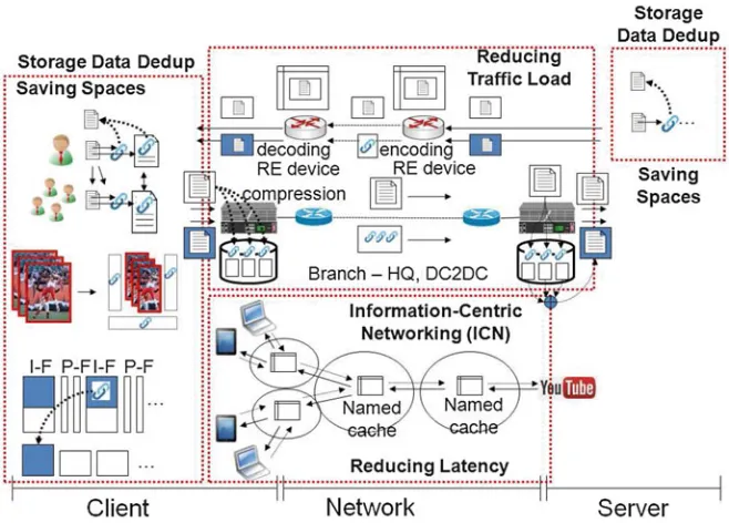
Fig. 1.3 Existing solutions to remove redundancies

The second approach to removing redundancies is called redundancy elimination (RE). With this approach the aim is to reduce traffic loads in networks. The typical example is the wide area network (WAN) optimizer that removes redundant network transfers between branches (or a branch) to a headquarter and one data centre to another. The WAN optimizer works as follows. Suppose a user sends a file to a remote server. Before the file moves through the network, the WAN optimizer splits the file into chunks and saves the chunks and corresponding indexes. The file is compressed and delivered to the WAN optimizer on the other side, where the file is again split into chunks that are saved along with the indexes. The next time the same file passes through the network, the WAN optimizer replaces it with small indexes. On the other side, the WAN optimizer reassembles the file with previously saved chunks based on indexes in a packet.

Another example is network-wide RE, which involves the use of a router (or switch) called a RE device. In this approach, for a unique transfer, the RE device saves the unique packets. When transfers become redundant, the RE device replaces the redundant payload within a packet with an index (called encoding) and reconstructs the encoded packet (called decoding).

(20)

a long processing time and high index overhead. Second, RE entails resource-intensive operations, such as fingerprinting, encoding and decoding at routers. Additionally, a representative RE study proposed a control module that involves a traffic matrix, routing policies and resource configurations, but few details are given, and some of those details are based on assumptions. Thus, we need to have an efficient way to adapt RE devices to dynamic changes. Third, ICN uses name-based forwarding tables that grow much faster than IP forwarding tables. Thus, long table-lookup times and scalability issues arise.

1.5 Deduplication Framework

To resolve (or reduce) issues of the existing solutions, an approach suggested in this book is to develop a deduplication framework that optimizes data from clients to servers throughout networks. The framework consists of three components that have different levels of redundancy removal (Fig.1.4).

The client component removes local redundancies from a client and is basically comprised of functions to decompose and reconstruct files. These components

(21)

8 1 Introduction

Fig. 1.5 Components developed for deduplication framework

should be fast and have low overhead considering the low capacity of most clients. The network component removes redundant transfers from different clients. In this component, the RE devices intercept data packets and eliminate redundant data. RE devices are dynamically controlled by software-defined network (SDN) controllers. This component should be fast when analysing large numbers of packets and be scalable to a large number of RE devices. Finally, the server component removes redundancies from different networks. This component should provide high space savings. Thus, fine-grained deduplication and fast responses are fundamental functions.

This book discusses practical implementations of the components of a deduplica-tion framework (Fig.1.5). For the server component, a Hybrid Email Deduplication System (HEDS) is presented. The HEDS achieves a balanced trade-off between space savings and overhead for email systems. For the client component, Structure-Aware File and Email Deduplication for Cloud-based Storage Systems (SAFE) is shown. The SAFE is fast and provides high storage space savings through structure-based granularity. For the network component, Software-Defined Deduplication as a Network and Storage Service (SoftDance) is presented. SoftDance is an in-network deduplication approach that chains storage data deduplication and redundancy elimination functions using SDN and achieves both storage space and network bandwidth savings with low processing time and memory overhead. Mobile deduplication is a client component that removes redundancies of popular files like images and video files on mobile devices.

1.6 Redundant Array of Inexpensive Disks

(22)

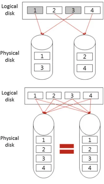
Fig. 1.7 RAID 1 (mirroring)

left disk, while blocks 2 and 4 are saved to the right disk. Because of independent parallel access to blocks on different disks, RAID 0 increases the read performance on the disks. RAID 0 could also make a large logical disk with small physical disks. However, the failure of a disk results in the loss of all data.

RAID 1 focuses on fault tolerance by mirroring blocks between disks (Fig.1.7). The left and right blocks have the same blocks (blocks 1, 2, 3, and 4). Even if one disk fails, RAID 1 can recover the lost data using blocks on the other disk. RAID 1 increases read performance owing to parallel access but decreases write performance owing to the creation of duplicates. RAID 5 uses block-level striping with distributed parity. As shown in Fig.1.8, each disk contains a parity representing blocks: for example, Cp is a parity for C1 and C2. RAID 5 requires at least three disks. RAID 5 increases read and write performance and fault tolerance.

1.7 Direct-Attached Storage

(23)

10 1 Introduction

Fig. 1.8 RAID 5 (Block-level striping with distributed parity

Fig. 1.9 Direct-attached storage (DAS)

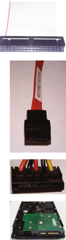
be inserted. DAS is mainly used to run applications on a computer. The first DAS interface standard was called Parallel Advanced Technology Attachment (PATA) and is used for hard disk drives, optical disk drives and floppy disk drives. In PATA, data are transferred from/to a storage device through a 16-bit wide cable. Figure1.10 shows a PATA data cable. The PATA cable supports various data rates, including 16, 33, 66, 100 and 133 MB/s.

PATA was replaced by Serial ATA (SATA) (Fig.1.11), which has faster speeds – 150, 300, 600 and 1900 MB/s – than PATA. SATA uses a serial cable (Fig.1.13). Figure1.12shows a power cable adapter for a SATA cable. Hard disks that support SATA provide a 7-pin data cable connector and a 15-pin power cable connector (Fig.1.13).

1.8 Storage Area Network

(24)

Fig. 1.11 SATA (Serial ATA) data cable

Fig. 1.12 Serial Advanced Technology Attachment (SATA) power cable

Fig. 1.13 SATA connectors: 7-pin data and 15 power connectors

(25)

12 1 Introduction

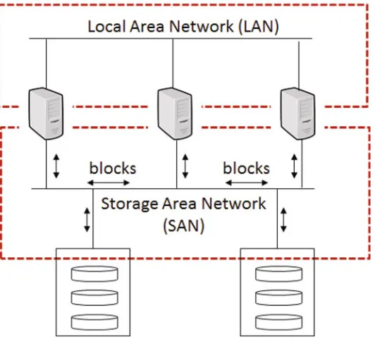
Fig. 1.14 Storage area network

send blocks (rather than files) to storage, and each storage device is shown to the application servers as if the storage were a hard disk drive like DAS.

A SAN has two main attributes. One is availability, the other is scalability. Stor-age data should be recoverable after a failure without having to stop applications. Also, as the number of disks increases, performance should increase linearly (or more). SAN protocols include Fibre Channel (FC), Internet Small Computer System Interface (iSCSI), and ATA over Ethernet (AoE).

1.9 Network-Attached Storage

Network-attached storage (NAS) refers to a computer that serves as a remote file server. While a SAN delivers blocks through a dedicated network, NAS, with disk arrays, receives files through a LAN, through which application data flow. As shown in Fig.1.15, application servers send files to NAS servers that subsequently save the received files to disk arrays. NAS uses file-based protocols such as Network File System (NFS), Common Internet File System (CIFS), and Andrew File System (AFS).

(26)

a browser-based configuration and management based on an IP address. As more capacity is needed, NAS servers support clustering and provide extra capacity by collaborating with cloud storage providers.

1.10 Comparison of DAS, NAS and SAN

The three types of storage system DAS, NAS, and SAN have different character-istics (Table1.1). Data storage in DAS is owned by individual computers, but in NAS and SAN it is shared by multiple computers. Data in DAS are transferred to data storage directly through I/O cables, but data using NAS and SAN should be transferred through a LAN for NAS and a fast storage area network for SAN. Data units to be transferred to storage are sectors on hard disks for DAS, files for NAS and blocks for SAN. DAS is limited in terms of the number of disks owing to the space on the computer and operators need to manage data storage independently on each computer. By contrast, SAN and NAS can have centralized management tools and can increase the size of data storage easily by just adding storage devices.

1.11 Storage Virtualization

(27)

14 1 Introduction

Table 1.1 Comparison of DAS, NAS and SAN

DAS NAS SAN

Shared(?) Individual Shared Shared

Network Not required Local area network Storage area network Protocols PATA, SATA NFS, CIFS, AFS Fibre Channel, iSCSI,

AoE

Data unit Sector File Block

Capacity Low Moderate/High High Complexity Easy Moderate Difficult Management High Moderate Low

has a common name, where the physical storage can be complex with multiple networks. Storage virtualization has multiple benefits, as follows:

• Fast provisioning: available free storage space is found rapidly by storage vir-tualization. By contrast, without storage virtualization, operators should find the available storage that encompasses enough space for the requested applications. • Consolidation: without storage virtualization, some spaces in individual storage

can be wasted because the remaining spaces are insufficient for applications. However, storage virtualization combines the multiple remaining spaces that are created as a logical storage space. Thus, spaces are efficiently utilized.

• Reduction of management costs: the number of operators that assign storage space for requested applications is reduced.

Software-defined storage (SDS) [1] has emerged as a form of software-based storage virtualization. SDS separates storage hardware from software and controls physically disparate data storage devices that are made by different storage compa-nies or that represent different storage types, such as a single disk or disk arrays. SDS is an important component of a software-defined data centre (SDDC) along with software-defined compute and software-defined networks (SDN).

(28)

Fig. 1.16 Big picture of SDS [1]

1.12 In-Memory Storage

In-memory storage or in-memory database (IMDB) has been developed to cope with the fast saving and retrieving of data to/from databases. Traditionally a database resides on a hard disk, and access to the disk is constrained by the mechanical movement of the disk head. Using a solid-state disk (SSD) or memory rather than disk as a storage device will result in an increase in the speed of data write and read. The explosive growth of of big data requires fast data processing in memory. Thus,IMDB is becoming popular for real-time big data analysis applications.

(29)

16 1 Introduction

1.13 Object-Oriented Storage

Object-oriented storage saves data as objects, whereas block-based storage stores data as fixed-size blocks. Object storage abstracts lower layers of storage, and data are managed objects instead of files or blocks. Object storage provides addressing and identification of individual objects rather than file name and path. Object storage separates metadata and data, and applications access objects through an application program interface (API), for example, RESTful API. In object storage, administrators do not have to create and manage logical volumes to use disk capacity.

Lustre [8] is a parallel distributed file system using object storage. Luster consists of compute nodes (Lustre clients), Lustre object storage servers (OSSs), Lustre object storage targets (OSTs), Lustre metadata servers (MDSs) and Luster metadata targets (MDTs). A MDS manages metadata such as file names and directories. A MDT is a block device where metadata are stored. An OSS handles I/O requests for file data, and an OST is a block device where file data are stored. OpenStack Swift [11] is object-based cloud storage that is a distributed and consistent objec-t/blob store. Swift creates and retrieves objects and metadata using the Object Stor-age RESTful API. This RESTful API makes it easier for clients to integrate Swift service into client applications. With the API, the resource path is defined based on a format such as /v1/{account}/{container}/{object}. Then the object can be retrieved at a URL like the following: http://server/v1/{account}/{container}/{object}.

1.14 Standards and Efforts to Develop Data Storage Systems

In this section, we discuss the efforts made and standards developed in the evolution of data storage. We start from a SATA and RAID. Then we explain a FC standard (FC encapsulation), iSCSI and Internet Fibre Channel Protocol (iFCP) for a SAN, and a NFS for NAS. We end by explaining the content deduplication standard and Cloud data management interface.

(30)

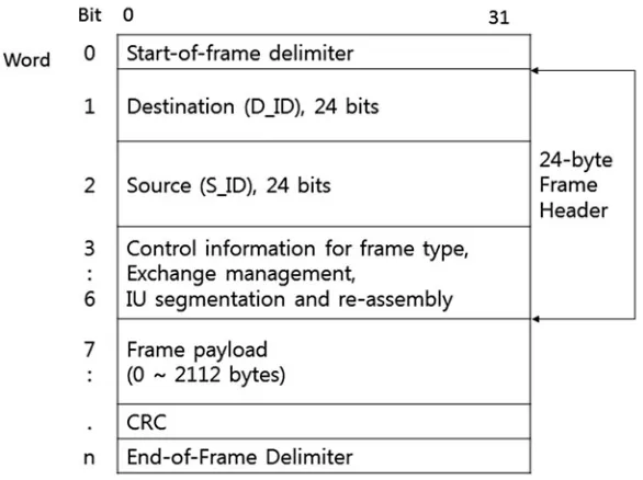
Fig. 1.17 Fibre Channel frame format

Patterson et al. [13] proposed a method, called RAID, to improve I/O perfor-mance by clustering inexpensive disks; this represents an alternative to single large expensive magnetic disks (SLEDs). Each disk in a RAID has a short mean time to failure (MTTF) compared to high-performance SLEDs. The paper focuses on the reliability and price performance of disk arrays, which shortens the mean time to repair (MTTR) due to disk failure by having redundant disks. When a disk fails, another disk replaces it. RAID 1 mirrors disks that duplicate all disks. RAID 2 uses hamming code to check and correct errors, where data are interleaved across disks and a sufficient number of check disks are used to identify errors. RAID 3 uses only one check disk. RAID 4 saves a data unit to a single sector, improving the performance of small transfers owing to parallelism. RAID 5 does not use separate check disks but distributes parity bits to all disks.

(31)

18 1 Introduction

Fig. 1.18 Small Computer System Interface architecture: interaction between client and server: cited from [19]

The SCSI architecture [19] is an interface for saving data to I/O devices and is defined in ANSI INCITS 366-2003 and ISO/IEC 14776-412. As shown in Fig.1.18, the application client within an initiator device (like a device driver) sends the SCSI commands to the device server in a logical unit located in a target device. The device server processes the SCSI commands and returns a response to the initiated client. The task manager receives and processes the task management requests, responding to the client as well. An application client sends requests by a remote procedure with input parameters, including command descriptor blocks (CDBs). CDBs are command parameters that define the operations to be performed by the device server. The iSCSI architecture is defined in RFC 7143 [2], where the SCSI runs through the TCP connections on an IP network. This allows an application client in an initiator device to send commands and data to a device server on a remote target device on a LAN, WAN, or the Internet. iSCSI is a protocol of a SAN but runs on an IP network without the need for special cables like FC. The application client communicates with the device server through a session that consists of one or more TCP connections. A session has a session ID. Likewise, each connection in the session has a connection ID. Commands are numbered in a session and are ordered over multiple connections in the session.

(32)

Fig. 1.19 Internet Fibre Channel Protocol (iFCP): cited from RFC 4172 [10]

The NFS that is defined in RFC 7530 [16] is a distributed file system, which is widely used in NAS. NFS is based on the Open Network Computing (ONC) Remote Procedure Call (RPC) (RFC 1831) [18]. The “Network File System (NFS) Version 4 External Data Representation Standard (XDR) Description” (RFC 7531) [3] defines XDR structures used by NFS version 4. NFS consists of a NFS server and NFS client: the NFS server runs a daemon on a remote server where a file is located and the NFS client accesses the file on the remote server using RPC. NFS provides the same operations on the remote files as those on the local files. When an application needs a remote file, the application opens a remote file to obtain access, reads data from the file, writes data to the file, seeks specified data in the file and closes the file when the application finishes. NFS is different from a file transfer service because the application does not retrieve and store the entire file but rather transfers small blocks of data at a time.

(33)

20 1 Introduction

Fig. 1.20 Content delivery network interconnection (CDNi): content naming mechanism, cited from [7]

located in multiple locations. Figure1.20shows the relationship between a content identifier and resource identifiers. The content identifier should be globally unique.

1.15 Summary and Organization

In this chapter, we have presented a deduplication framework that consists of a client, server and network components. We also illustrated the evolution of data storage systems. Data storage has evolved from a single hard disk attached to a single computer by DAS. As the amount of data increases and large amounts of storage are required for multiple computers, storage is located in different places where data are shared from multiple computers (including application servers) by a SAN or NAS. To increase the read or write performance and fault tolerance, RAIDs are used with different levels of services, including striping, mirroring or striping with distributed parity. SDS, which is a critical component of a SDDC, consolidates and virtualizes disparate data storage devices using storage/service pools, data service, SDS API and data management API.

(34)

Representation Standard (XDR) Description.https://tools.ietf.org/html/rfc7531(2015) 4. Hazelcast.org: Hazelcast.http://hazelcast.org/(2016)

5. IBM: eXtremeScale.http://www-03.ibm.com/software/products/en/websphere-extreme-scale (2016)

6. IDC: The digital universe in 2020. https://www.emc.com/collateral/analyst-reports/idc-the-digital-universe-in-2020.pdf(2012)

7. Jin, W., Li, M., Khasnabish, B.: Content De-duplication for CDNi Optimization.https://tools. ietf.org/html/draft-jin-cdni-content-deduplication-optimization-04(2013)

8. lustre.org: Lustre.http://lustre.org/(2016)

9. Meyer, D.T., Bolosky, W.J.: A study of practical deduplication. In: Proceeding of the USENIX Conference on File and Storage Technologies (FAST) (2011)

10. Monia, C., Mullendore, R., Travostino, F., Jeong, W., Edwards, M.: iFCP - A Protocol for Internet Fibre Channel Storage Networking.http://www.rfc-editor.org/info/rfc4172(2005) 11. openstack.org: OpenStack Swift. http://www.openstack.org/software/releases/liberty/

components/swift(2016)

12. Oracle: Coherence. http://www.oracle.com/technetwork/middleware/coherence/overview/ index.html(2016)

13. Patterson, D.A., Gibson, G., Katz, R.H.: A case for redundant arrays of inexpensive disks (raid). In: Proceedings of the 1988 ACM SIGMOD International Conference on Management of Data, SIGMOD ’88 (1988)

14. Serial_ATA: Fast Just Got Faster: SATA 6Gb/s. https://www.sata-io.org/system/files/member-downloads/SATA-6Gbs-Fast-Just-Got-Faster_2.pdf(2009)

15. Serial_ATA: SATA revision 3.2 specification. https://www.sata-io.org/sites/default/files/ documents/SATA_v3%202_PR__Final_BusinessWire_8.20.13.pdf(2013)

16. Shepler, S., Callaghan, B., Robinson, D., Thurlow, R., Beame, C., Eisler, M., Noveck, D.: Network File System (NFS) Version 4 Protocol.http://www.rfc-editor.org/info/rfc7530(2015) 17. Spring, N.T., Wetherall, D.: A protocol-independent technique for eliminating redundant net-work traffic. In: Proceedings of the ACM SIGCOMM 2000 conference on Data communication (2000)

18. Srinivasan, R.: RPC: Remote Procedure Call Protocol Specification Version 2. https://tools. ietf.org/html/rfc1831(1995)

19. T10, I.T.C.: SCSI Architecture Model-2 (SAM-2). ANSI INCITS 366-2003, ISO/IEC 14776-412 (2003)

20. VMWare: Gemfire.https://www.vmware.com/support/pubs/vfabric-gemfire.html(2016) 21. Weber, R., Rajagopal, M., Travostino, F., O’Donnell, M., Monia, C., Merhar, M.: Fibre Channel

(35)

Chapter 2 Existing Deduplication Techniques

Abstract Though various deduplication techniques have been proposed and used, no single best solution has been developed to handle all types of redundancies. Considering performance and overhead, each deduplication technique has been developed with different designs considering the characteristics of data sets, system capacity and deduplication time. For example, if the data sets to be handled have many duplicate files, deduplication can compare files themselves without looking at the file content for faster running time. However, if data sets have similar files rather than identical files, deduplication should look inside the files to check what parts of the contents are the same as previously saved data for better storage space savings. Also, deduplication should consider different designs of system capacity. High-capacity servers can handle considerable overhead for deduplication, but low-capacity clients should have lightweight deduplication designs for fast performance. Studies have been conducted to reduce redundancies at routers (or switches) within a network. This approach requires the fast processing of data packets at the routers, which is of crucial necessity for Internet service providers (ISPs). Meanwhile, if a system removes redundancies directly in a write path within a confined storage space, it is better to eliminate redundant data before storage. On the other hand, if a system has residual (or idle) time or enough space to store data temporarily, deduplication can be performed after the data are placed in temporary storage. In this chapter, we classify existing deduplication techniques based on granularity, place of deduplication and deduplication time. We start by explaining how to efficiently detect redundancy using chunk index caches and bloom filters. Then we describe how each deduplication technique works along with existing approaches and elaborate on commercially and academically existing deduplication solutions. All implementation codes are tested and run on Ubuntu 12.04 precise.

2.1 Deduplication Techniques Classification

Deduplication can be divided based on granularity (the unit of compared data), deduplication place, and deduplication time (Table2.1). The main components of these three classification criteria are chunking, hashing and indexing. Chunking is a process that generates the unit of compared data, called a chunk. To compare

D. Kim et al.,Data Deduplication for Data Optimization for Storage and Network Systems, DOI 10.1007/978-3-319-42280-0_2

(36)

duplicate chunks, hash keys of chunks are computed and compared, and a hash key is saved as an index for future comparison with other chunks.

Deduplication is classified based on granularity. The unit of compared data can be at the file level or subfile level, which are further subdivided into fixed-size blocks, variable-sized chunks, packet payload or byte streams in a packet payload. The smaller the granularity used, the larger number of indexes created, but the more redundant data are detected and removed.

For place of deduplication, deduplication is divided into server-based and client-based deduplication for end-to-end systems. Server-based deduplication tra-ditionally runs on high-capacity servers, whereas client-based deduplication runs on clients that normally have limited capacity. Deduplication can occur on the network side; this is known asredundancy elimination(RE). The main goal of RE techniques is to save bandwidth and reduce latency by reducing repeating transfers through the network links. RE is further subdivided into end-to-end RE, where deduplication runs at end points on a network, and network-wide RE (or in-network deduplication), where deduplication runs on network routers.

In terms of deduplication time, deduplication is divided into inline and offline deduplication. With inline deduplication, deduplication is performed before data are stored on disks, whereas offline deduplication involving performing deduplication after data are stored. Thus, inline deduplication does not require extra storage space but incurs latency overhead within a write path. Covnersely, offline deduplication does not have latency overhead but requires extra storage space and more disk bandwidth because data saved in temporary storage are loaded for deduplication and deduplicated chunks are saved again to more permanent storage. Inline dedu-plication mainly focuses on latency-sensitive primary workloads, whereas offline deduplication concentrates on throughput-sensitive secondary workloads. Thus, inline deduplication studies tend to show trade-offs between storage space savings and fast running time.

(37)

2.2 Common Modules 25

2.2 Common Modules

2.2.1 Chunk Index Cache

Deduplication aims to find as many redundancies as possible while maintaining processing time. To reduce processing time, one typical technique is to check indexes of data in memory before accessing disks. If the data indexes are the same, deduplication does not involve accessing the disks where the indexes are stored, which would reduce processing time. An index represent essential metadata that are used to compare data (or chunks). In this section, we show what can be indexed and how indexes are computed, stored and used for comparisons.

2.2.1.1 Fundamentals

To compare redundant data, deduplication involves the computation of data indexes. Thus, an index should be unique for all data with different content. To ensure the uniqueness of an index, one-way hash functions, such as message digest 5 (MD5), secure hash algorithm 1 (SHA-1), or secure hash algorithm 2 (SHA-2) are used. These hash functions should not create the same index for different data. In other words, an index is normally considered a hash key that represents data. Indexes should be saved to permanent storage devices like a hard disk, but to speed up the comparison of indexes, they are prefetched in memory. The indexes in memory should provide temporal locality to reduce the number of evictions of indexes from memory owing to filled memory as well as a decrease in the number of prefetches. In the same sense, to prefetch related indexes, the indexes should be grouped by spatial locality. That is, indexes of similar data are stored close to each other in storage.

An index table is a place where indexes are temporarily located for fast comparison. Such tables can be deployed using many different methods, but mainly they are built using hash tables, which allows comparisons to be made very quickly due to the time complexity of O(1) with the overhead of hash table size. In the next section, we present a simple implementation of an index table using an unordered_map container.

2.2.1.2 Implementation: Hash Computation

(38)

We provide a main function to test the computation of a hash key and a Makefile to make compilation easy. In the main function, the first paragraph shows how to compute a hash key of a file, and the second paragraph shows how to calculate a hash key of a string block:

# i f d e f SHA 1WRAPPER_TEST

i n t main ( ) {

Sha1Wrapper o b j ;

s t r i n g f i l e P a t h = " h e l l o . d a t " ;

s t r i n g d a t a = " h e l l o danny how a r e you ? ? " ;

s t r i n g hashKey ;

/ / g e t h a s h k e y o f a f i l e

hashKey = o b j . g e t H a s h K e y O f F i l e ( f i l e P a t h ) ;

c o u t << " h a s h k e y o f " << f i l e P a t h << " : " << hashKey << e n d l ; c o u t << e n d l ;

/ / g e t h a s h k e y o f d a t a c o u t << d a t a << e n d l ;

hashKey = o b j . g e t H a s h K e y ( d a t a ) ;

c o u t << " h a s h k e y o f d a t a : " << hashKey << e n d l ;

r e t u r n 0 ; }

# e n d i f

## make a l l :

g++ DSHA1WRAPPER_TEST o SHA 1 s h a 1 . c c s h a 1 W r a p p e r . c c

c l e a n :

rm f . o SHA 1

We compile and build an executable file to test SHA-1 as follows:

r o o t @ s e r v e r : ~ / l i b / SHA 1# make

g++ DSHA1WRAPPER_TEST o SHA 1 s h a 1 . c c s h a 1 W r a p p e r . c c r o o t @ s e r v e r : ~ / l i b / s h a 1 # l s l

(39)

rw r r 1 r o o t r o o t 20297 J u l 20 2 0 : 2 8 s h a 1 . c c rw r r 1 r o o t r o o t 4606 J u l 20 2 0 : 2 8 s h a 1 . h

rw r r 1 r o o t r o o t 1187 J u l 20 2 0 : 2 8 s h a 1 W r a p p e r . c c rw r r 1 r o o t r o o t 522 J u l 20 2 0 : 2 8 s h a 1 W r a p p e r . h

Following are the results of running a SHA-1 executable file. We retrieve an index string with 40 characters created from 20 bytes; 1 byte is denoted by two hexadecimals. Thus, the size of the index amounts to 40 bytes (40 characters). The first hash key that starts with 49a32. . . is computed from a file (here, hello.dat). The second hash key starting with e69927 is computed from a string “hello danny how are you??”:

We show an implementation of an index table using an unordered_map. The imple-mentation codes are in AppendixB. We compile and build a cache executable file. To compile using an unordered_map, we need to add ‘-std=c++0x’ at compilation:

r o o t @ s e r v e r : ~ / l i b / c a c h e # make

(40)

c o u t << " c u r r e n t c a c h e " << e n d l ;

(41)

‘sizeOfAll-2.2 Common Modules 29

EntriesDouble()’, ‘sizeOfKeys()’, ‘sizeOfKeysDouble()’ and ‘sizeOfValues()’. That is, ‘cache.sizeOfAllEntriesDouble()’ shows the size of the index table, including all pairs; ‘cache.sizeOfKeys()’ and ‘cache.sizeofValues()’ return the size of keys or values in the index table respectively; ‘cache.sizeOfKeysDouble()’ and ‘cache.sizeOfValuesDouble’ return the size of double data type; and ‘cache.removeAll()’ removes all indexes in the index table.

/ / show a l l e n t r i e s

(42)

show a l l e n t r i e s 1 , Danny

2 , Kim

s i z e o f a l l e n t r i e s ( b y t e s ) : 10

s i z e o f a l l e n t r i e s (d o u b l e v a l u e ) ( b y t e s ) : 10 s i z e o f k e y s ( b y t e s ) : 2

s i z e o f k e y s (d o u b l e v a l u e ) ( b y t e s ) : 2 s i z e o f v a l u e s ( b y t e s ) : 8

_{remove a l l} _{e n t r i e s} s i z e o f a l l e n t r i e s : 0

2.2.2 Bloom Filter

To prevent an index table occupying memory as the number of indexes grows in the index table, a small summary vector, called a Bloom filter, is used to quickly check whether data are unique using small sized metadata. In this section, we see how Bloom filter codes are implemented.

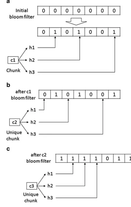
A Bloom filter is used to see whether duplicate chunks of data exist in storage. The Bloom filter is a bit array ofmbits initially set to 0. Given a setU, each elementu (u 2U) of the set is hashed usingkhash functionsh1; : : : ;hk. Each hash function

hi.u/returns an array index in the bit array that ranges from 0 tom 1. Subsequently,

a bit of the index is set to 1. This Bloom filter is used to check whether an element was already saved to a set. When an element attempts to be added to a set, if one of the bits corresponding to the return values of hash functionsh1; : : : ;hkis 0, then the

element is considered a new one in the set. If bits corresponding to return values of hash functions are all 1, the element is considered to exist in the set.

(43)

Fig. 2.1 How the Bloom filter works. (a) Bloom filter after c1 chunk is saved. (b) Bloom filter when c2, a unique chunk, is compared. (c) Bloom filter when c3, a unique chunk, is compared (false positive). A unique chunk is found to be redundant

(44)

of hash functions. To achieve a 2 % false positive, the smallest size of the Bloom filter ism= 8 *nbits (m/n= 8), and the number of hash functions is four. Thus, we compute the size of the Bloom filter bit array (m) to 1280 bits as follows. We choose 1283 rather than 1280 for the size of the Bloom filter bit array because the prime number shows a good uniform distribution, reducing the primary cluster as shown in Weiss’ book [47] when the mod() function is used for the hash function:

n = 160 b i t s (SHA 1 h a s h key ) m = 8 160 = 1280 b i t s k = 4 ( f o u r h a s h f u n c t i o n s )

The codes are compiled and built by typing ‘make’, and bf is the executable file used to test the Bloom filter codes:

r o o t @ s e r v e r : ~ / b f # make

g c c DBF_TEST DDEBUG o b f b f . c

r o o t @ s e r v e r : ~ / b f # l s l

rwxr xr x 1 r o o t r o o t 12861 J u l 21 0 8 : 5 9 b f rw r r 1 r o o t r o o t 5627 J u l 21 0 0 : 3 9 b f . c rw r r 1 r o o t r o o t 1585 J u l 21 0 0 : 3 8 b f . h rw r r 1 r o o t r o o t 51 J u l 21 0 8 : 5 9 M a k e f i l e

Following are the results of the testing program of the Bloom filter codes. First, we assign two fingerprints (which are considered to be hash keys). The Bloom filter is initialized with a bit array with all 0s in each bit. We use 11 bits for the Bloom filter; readers can extend the size if needed. When data with the first hash key (fingerpt1) are saved, deduplication checks the Bloom filter. The bit indexes that four hash functions compute are 2, 4, 7 and 8. Please note that the bit index starts at 0. The data are found to be unique because 0 is found among the bit values. Then the values of the bit indexes (2, 4, 7, 8) are changed to 1, and the Bloom filter has 00101001100 bit arrays:

r o o t @ s e r v e r : ~ / b f # b f

## # # # # # # # # # # # # # # # # # # # # # # # # # # # # # # # # T e s t : I n p u t D a t a ## ## # # # # # # # # # # # # # # # # # # # # # # # # # # # # # # #

[ bloom f i l t e r ] f i n g e r p t 1 : 4543863031426141731 [ bloom f i l t e r ] f i n g e r p t 2 : 4543863041425141743

## # # # # # # # # # # # # # # # # # # # # # # # # # # # # # # # [ bloom f i l t e r ] i n i t i a l i z e

(45)

(46)

calculate the 1, 4, 7 and 8 bit indexes. Though the bit values of the 4, 7, 8 indexes are found to be 1, the bit values of the 1 bit index (second bit) is still 0. This means the current data are unique. Therefore, the Bloom filter says the current data do not exist in the previously saved data. Then the bit value of the 1 bit index (second bit) is changed to 1.

2.3 Deduplication Techniques by Granularity

2.3.1 File-Level Deduplication

File-level deduplication uses file-level granularity, which is the most coarse-grained granularity. File-level deduplication compares entire files based on a hash value of a file, like SHA-1 [34], to avoid saving the same files. In this section, we demonstrate how file-level deduplication works and its implementation.

We begin by explaining how file-level deduplication works. As shown in Fig.2.2, suppose we have two identical files. When we save the first file, deduplication computes an index that is a hash value using a one-way hash function. If the index is not found in the index table, the file is unique. In this case, the index and the file are saved to the index table and storage respectively. For the second file, the index of the file is found in the index table, so the corresponding file is not saved.

(47)

2.3 Deduplication Techniques by Granularity 35

Fig. 2.2 File-level deduplication

simple file-level deduplication can achieve three-quarters of the space savings of aggressive, expensive block deduplications (to be discussed in the next two sections) at a lower cost in terms of performance and complexity.

2.3.1.2 Implementation

The first step of file-level deduplication is to compute an index (hash key) of a file, and the hash key and data of the file are fed into a file-level deduplication function, called the dedupFile(). The SHA-1 hash key is used as an index computed by the getHashKey() with the data of the file:

F i l e O p e r f i l e O p e r ; Sha1Wrapper s h a 1 W r a p p e r ; s t r i n g d a t a , hashKey ;

d a t a = f i l e O p e r . g e t D a t a ( f i l e P a t h ) ; / / p a t h o f t h e f i l e t o be s a v e d

hashKey = s h a 1 W r a p p e r . g e t H a s h K e y ( d a t a ) ;

d e d u p F i l e ( hashKey , d a t a ) ;

getData() in FileOper class read a file and load the content to a string typed variable. getData() is implemented using ifstream() as follows:

s t r i n g

F i l e O p e r : : g e t D a t a ( s t r i n g f i l e P a t h ) {

s t r i n g r e s u l t , l i n e ;

i f s t r e a m f i l e ( (c h a r) f i l e P a t h . c _ s t r ( ) ) ; i f ( f i l e . i s _ o p e n ( ) ) {

w h i l e ( f i l e . good ( ) ) { g e t l i n e ( f i l e , l i n e ) ; i f ( ! f i l e . e o f ( ) )

r e s u l t += l i n e + " \ n " ; e l s e

(48)

The dedupFile() function begins by comparing the hash key in arguments with pre-existing indexes in a hash table, checking whether data corresponding to the hash key are unique or duplicates. In code, we use a flag variable, called ‘isUnique’, that has ‘false’ initially. File-level deduplication checks the Bloom filter with an index (hash key). If the Bloom filter returns ‘true’, then we further check the chunk index cache because there may be false positives. If the Bloom filter returns ‘false’, the current data are determined to be unique with 100 % certainty, and ‘isUnique’ is changed to ‘true”:

v o i d

SDedup : : d e d u p F i l e ( s t r i n g f i l e H a s h K e y , s t r i n g d a t a ) {

b o o l e a n i s U n i q u e = f a l s e;

/ /

/ / c h e c k bloom f i l t e r / /

i f ( e x i s t I n B l o o m F i l t e r ( f i l e H a s h K e y ) ) {

/ / due t o f a l s e p o s i t i v e , we c h e c k c h u n k i n d e x s u b s e q u e n t l y .

/ /

/ / c h e c k c h u n k i n d e x c a c h e / /

/ / d u p l i c a t e d a t a

i f ( ! i s D u p l i c a t e I n C a c h e ( f i l e H a s h K e y ) ) { i s U n i q u e = t r u e;

} } e l s e {

i s U n i q u e = t r u e; }

i f ( i s U n i q u e ) {

s a v e I n C a c h e ( f i l e H a s h K e y ) ;

/ / s a v e t o s t o r a g e

sm . s e t B u f f e r e d D a t a ( f i l e H a s h K e y , d a t a ) ; }

}

(49)

If the current data are determined to be unique by the Bloom filter or chunk index cache, the index is saved to the chunk index cache using the saveInCache() function. ‘sm.setBufferedData(fileHashKey, data)’ buffers data contents, compresses the data, and saves them to storage. ‘sm’ is an object of the ‘StoreManager’ class.

2.3.1.3 Existing Solutions

File-level deduplication is used for Microsoft Exchange 2003 and 2007 based on a SIS [5]. SIS stores file contents to a ‘SIS Common Store’. In SIS, a user file is managed by a SIS link that is a reference to a file called the ‘Common Store File’. Whenever SIS detects duplicate files, SIS links are created automatically and file contents are saved to the common store. SIS consists of a file system filter library that implements links and a user-level service detecting duplicate files that are replaced by links. SIS can find duplicate files but not large redundancies within similar files. We address this issue by developing the Hybrid Email Deduplication System (HEDS) [23].

File-level deduplication is used for popular cloud storage systems, such as JustCloud [22] and Mozy [32], to reduce latency in a client. Cloud storage system client applications run file-level deduplication that computes an index (hash key) of each file and checks whether the index exists in a server. If the server has the index, the client does not send the duplicate file. Running the file-level deduplication in the client before sending data to a server allows cloud storage systems to consume less storage space and bandwidth. One study [20] measured the performance of several cloud storage systems including Mozy.

(50)

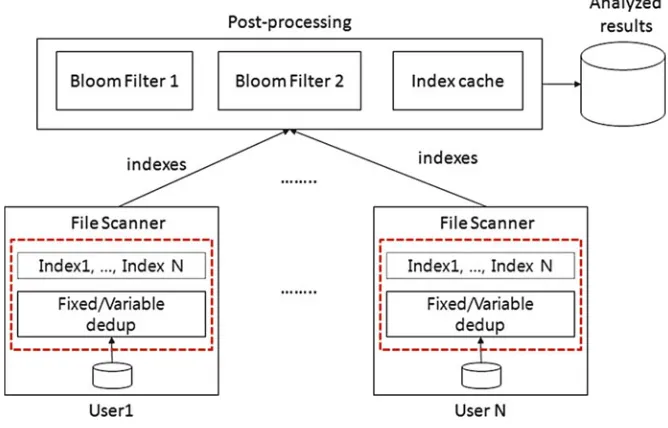
Fig. 2.3 A study of practical deduplication: evaluation set-up

maximum chunk sizes, 4 KB and 128 KB respectively. The expected chunk size ranges from 8 to 64 KB. The computed indexes are collected by a post-processing module that checks the redundancies of indexes using two Bloom filters. The size of each Bloom filter is 2 GB. The analysed results are saved to a database. The computed total size of the files is 40 TB, and the number of files is 200 million. File duplicates are found in post-processing by identifying files where all chunks matched. This study also mentions that a semantic knowledge of file structures would be useful to reduce redundancies with less overhead, and our Structure-Aware File and Email Deduplication for Cloud-based Storage Systems (SAFE) approach exploits the semantic information of file structures, as shown in Chap.4.

2.3.2 Fixed-Size Block Deduplication

(51)

Fig. 2.4 Fixed-size block deduplication

Fixed-size block-level deduplication separates a file into the same sized blocks and finds redundant blocks by comparing the indexes of the blocks. It runs fast because it only relies on offsets in a file to separate a file into blocks. However, fixed-size block deduplication has an issue when it comes to finding matching contents in similar files when the content at the beginning of the files is changed. For example, as shown in Fig.2.4, suppose deduplication uses a 15 byte fixed-size block as granularity. When we save an original fileFile1, deduplication splits the file into 15 byte fixed-size blocks. Likewise, when we save an updated file File2, in which we add the small text ‘welcome’ at the beginning of the original file, deduplication again splits the file into fixed-size blocks. However, blocks split from the updated second file are totally different from blocks split from the original first file. This is because the contents are shifted in the file; this is called theoffset-shifting problem.

Fixed-size block deduplication has been used for archival storage systems like Venti [39]. Venti uses fixed-size blocks as the granularity level and compares SHA-1 hash keys of blocks with previously saved hash keys following an on-disk index hierarchy. A popular cloud storage system, Dropbox [12], uses very large fixed-size (4 MB) block deduplication. Dropbox reduces network redundant traffic and redundant savings in the server by communicating with indexes between clients and servers before sending the data. Detailed information on how Dropbox works is explained in Chap.4.

2.3.2.2 Implementation

(52)

point to the array of blocks whose type is the string. We also need a variable, ‘numOfBlocks’, that shows the number of blocks in a file. The hashKey variable indicates the index of each block. In this code, the Bloom filter is not shown, but the checking of redundancy by the Bloom filter can be located before checking using the isDuplicateInCache() function with ‘chunk index cache’.

v o i d

SDedup : : d e d u p B l o c k ( s t r i n g f i l e H a s h K e y , s t r i n g d a t a , i n t b l k S i z e ) {

s t r i n g b l o c k s ; i n t numOfBlocks = 0 ; s t r i n g hashKey ; i n t i ;

/ /

/ / c h e c k d u p l i c a t e f i l e / /

/ / A d u p l i c a t e f i l e d o e s n o t n e e d t o be de d u p l i c a t e d t o b l o c k s

i f ( i s D u p l i c a t e I n C a c h e ( f i l e H a s h K e y ) ) { r e t u r n;

} e l s e {

s a v e I n C a c h e ( f i l e H a s h K e y ) ; }

/ /

/ / c h e c k d u p l i c a t e b l o c k s / /

/ / s e t b l o c k s i z e

c h u n k W r a p p e r . s e t A v g C h u n k S i z e ( b l k S i z e ) ;

/ / g e t b l o c k s f r o m a d a t a

b l o c k s = c h u n k W r a p p e r . g e t B l o c k s ( d a t a , numOfBlocks ) ;

f o r ( i = 0 ; i < numOfBlocks ; i ++) {

/ / g e t h a s h k e y o f a b l o c k

hashKey = s h a 1 W r a p p e r . g e t H a s h K e y ( b l o c k s [ i ] ) ;

(53)

In pure fixed-size block deduplication, a file is directly split into blocks without checking whether the file itself exists, causing redundant processing overhead and memory overhead. Thus, the dedupBlock() function first checks whether there is a duplicate file with an index of the current file. If a file is redundant, the file is not separated into blocks. An index of the file is saved to the index table using the saveInCache() function, and the dedupBlock() function ends.

(54)

The preceding code shows the getBlocks() function implementation. Please note that chunk and block terms are used interchangeably. In getBlocks(), the number of blocks is computed by dividing the size of the data by the block size (chunkSize). We maintain beginOffset and endOffset for each block, and each block is split from the data and ultimately contained in the string element of the chunk array using a substr() function. After all blocks are contained in a chunk string array, the reference variable of the chunks are returned.

2.3.2.3 Existing Solutions

Venti [39] is a fixed-size block deduplication system and uses a write-once policy, preventing data being inconsistent or causing malicious data loss. The main idea is that a file is divided into several blocks, and the index (hash key) of each block is created by a SHA-1 hash function. If the index of the block is the same as a previously saved index, the block is not saved. The index is arranged into a hash tree for reconstructing a file that contains the block. To improve performance, Venti uses three techniques: caching, striping and write buffering. The block and index are cached. Venti shows the possibility of using a hash key to differentiate each block in a file. Most deduplication applications that have been published split a file into several blocks (or chunks) and save each block based on the index (hash key) of each block.

Figure2.5shows how files are saved into the tree structure of Venti. A data block is pointed to by an index (hash key) of the block, and the indexes are packed into a pointer block with pointers. As shown in Fig.2.5a, Venti creates a hash key of a pointer blockP0 that is a root pointer block of file1. Venti creates new pointer blocksP1 andP2that subsequently point toD0,D1,D2andD3. Thus, data blocks

offile1are retrieved following on the tree structure of pointer blocks starting from

P0. Figure2.5b demonstrates how the tree structure is changed when a similar file

(file2) is saved. Supposefile2has two identical data blocks (D0 andD1), likefile1,

but two unique data blocks (D4andD5). Venti does not change the pointer blocks but instead creates new pointer blocks (P3andP4) forfile2.File2can be retrieved using pointer blocksP3,P1, andP4.

(55)

Fig. 2.5 Venti tree structure of data blocks [39]. (a) Tree structure of an original file (File1).File1 consists of four data blocks, includingD0;D1;D2;and D3. (b) Tree structure of a similar file (File2).File2consists of four data blocks, includingD0;D1;D4;and D5

We leverage SAFE into a Dropbox client to deduplicate structured files on the client side. Dropbox consists of two type of servers, one a control server and the other a storage server. Control servers hold metadata of files such as the hash value of individual blocks and mapping between a file and its blocks. Storage servers contain unique blocks in Amazon S3 [2]. Dropbox client synchronizes its own data and indexes with Dropbox servers.

(56)

Fig. 2.6 Dropbox internal mechanism

the following steps to save a file. (1) As soon as a user savesFile-Ato a shared folder in a Dropbox client, the fixed-size block deduplication of Dropbox splits the file into blocks based on 4 MB granularity and computes hashes of the objects. If a file is larger than 4 MB, then the file is the same as an object and a hash value of the file is computed. Dropbox uses SHA256 [35] to compute a hash value. (2–4) The Dropbox client sends all computed hash values of a file to a control server that returns only unique hash values after checking previously saved hash values. In this example, the hash key ofBlk-Bis returned to a client because the hash key ofBlk-A is found to be a duplicate. (5–6) The Dropbox client sends the blocks of returned indexes to the storage server. Ultimately, storage servers have unique blocks across all Dropbox clients. Note that storage saving occurs in a server (thanks to not saving

Blk-Aagain), and the incurred network load is reduced because onlyBlk-Bis sent.

2.3.3 Variable-Sized Block Deduplication

(57)

Fig. 2.7 Variable-sized block deduplication

Variable-sized block deduplication has been proposed to solve theoffset-shifting

problemof fixed-size block deduplication. Variable-sized block deduplication relies

on contents rather than a fixed offset. Figure2.7illustrates how variable-sized block deduplication works. Suppose we have two files.File1is an original file andFile2is an updated file in which we add brief texts in the middle of the file. When we save

File1, deduplication slides a small window from the beginning of the file. While the

window is sliding byte by byte, a fingerprint [40] of each window is computed and the two lowest digits are compared with a pre-defined value. If they are the same, the window is set to a chunk boundary. Then the contents ranging from the previous chunk boundary to the current chunk boundary is treated as a chunk. The window keeps sliding and finding chunk boundaries in the same manner. As a result, three unique chunks (C1,C2,C3) and the corresponding indexes are saved. When we save the updated second file, deduplication again slides a window and finds chunks. C4is found to be unique, andC1andC3are found to be redundant. Here, we see that chunk boundaries are maintained, though the contents are shifted in a file. Thus, content-based variable-sized block deduplication can find more redundancies than offset-based fixed-size block deduplication.

(58)

(59)

2.3.3.3 Implementation: Rabin Fingerprint

The Rabin fingerprint [40] is used to find chunk boundaries, resulting in the identification of a chunk. The Rabin fingerprint is a 64 bit key. When we compute fingerprints in data (byte stream using sliding windows), a fingerprint of each win-dow can be computed quickly based on the previous fingerprints using the following equation. Detailed information can be found in [43]. The full implementation codes are in AppendixD:

RF.tiC1: : :tˇCi/D.RF.ti: : :tˇCi 1/ tipˇ/CtˇCi modM: (2.1)

We can compile and build a test program to compute the Rabin fingerprint by typing ‘make’. The results from running the executable file, rabin, show a fingerprint (with long integer type) for the ‘hello tom danny’ string.

r o o t @ s e r v e r : ~ / r a b i n # make

Chunking is the first of three steps in deduplication (the other steps are hashing and indexing). The snippet codes for chunking are found in Appendix E. The core function in chunking is process_chunk in chunk_sub.cc. The process_chunk() function slides a small window byte by byte on the data, finds the chunk boundaries, and saves the beginning and ending indexes for all chunks to the ‘begin_indexes’ and ‘end_indexes’ integer arrays respectively. That is, the goal of the process_chunk() function is to identify the boundaries of the chunks. Based on the boundaries, the chunking Wrapper class, as shown in AppendixF, splits the data into chunks.

(60)

(61)

(62)

(63)

2.3.3.5 Implementation: Chunking Wrapper

The chunkWrapper class defines functions [getChunks()] to separate data into variable-sized chunks based on beginning and ending indexes computed by the chunking core class. The chunkWrapper class also defines functions to obtain fixed-size blocks [getBlocks()]. The chunkWrapper class requires other libraries, includ-ing the chunkinclud-ing core class (Sect.2.3.3.4), Rabin fingerprint class (Sect.2.3.3.3) and SHA-1 hashing (Sect.2.2.1.2). The chunkWrapper class also requires a file operation class based on the C++ Boost library. The file operation class is not shown in this book owing to the large code size.

(64)

rw r r 1 r o o t r o o t 52812 J u l 25 1 6 : 0 1 f i l e O p e r . c c rw r r 1 r o o t r o o t 22577 J u l 25 1 6 : 0 1 f i l e O p e r . h

We show three results obtained from running the program. The first variable-sized chunking extracts 14 chunks based on 8 KB (8192 bytes) average chunk size. Lines show the chunk boundaries and the chunk sizes after showing the boundaries. The second variable-sized chunking extracts 45 chunks from the same data. This is because an average chunk size (2 KB) that is smaller than the first chunking is used. The smaller the average chunk size used, the more chunks are created. The third result shows blocks extracted by getBlocks(), which means fixed-size blocks.

(65)

Variable-sized block deduplication involves expensive chunking and indexing for finding large redundancies, requiring an efficient in-memory cache and on-disk layout on high-capacity servers. DDFS [50] exploits three techniques to relieve a disk bottleneck, reducing processing time. A summary vector, which is a compact in-memory data structure, is used to find new data. Stream-informed segment layout, on-disk layout, is used to improve spatial locality for both data and indexes. The idea of a stream-informed segment layout is that a segment tends to reappear in similar sequences with other segments. This spatial locality is called segment duplicate

locality. Locality-preserved caching uses segment duplicate locality to acquire a

high hit ratio in the memory cache. The study removes 99 % of disk accesses and achieves 100 MB/s and 210 MB/s for single-stream throughput and multi-stream throughput respectively.

(66)

Fig. 2.8 Sparse indexing: deduplication process [26]

a sequence of chunks. A byte stream is split into chunks by Chunker using variable-sized chunking, and a sequence of chunks becomes a segment by Segmenter. Two segments are similar if they share a number of chunks. The Champion chooser chooses sampled segments, called champion, from a sparse index (in-memory index). Deduplicator compares chunks in incoming segments with chunks in champions (selected segments). Unique segments are saved to the sparse index for future comparison, and new chunks are saved to the Container store.

2.3.4 Hybrid Deduplication

Hybrid approacheshave been proposed by adaptively using variable-sized