With Big Data Applications
Stefania Loredana Nita
Marius Mihailescu
Practical
Concurrent
Practical Concurrent Haskell: With Big Data Applications
Stefania Loredana Nita Marius Mihailescu
Bucharest, Romania Bucharest, Romania
ISBN-13 (pbk): 978-1-4842-2780-0 ISBN-13 (electronic): 978-1-4842-2781-7 DOI 10.1007/978-1-4842-2781-7
Any source code or other supplementary material referenced by the author in this book is available to readers on GitHub via the book's product page, located at www.apress.com/9781484227800. For more detailed information, please visit http://www.apress.com/source-code.
Library of Congress Control Number: 2017953873
Contents at a Glance
■
Part I: Haskell Foundations. General Introductory Notions ...
1
■
Chapter 1: Introduction ...
3
■
Chapter 2: Programming with Haskell ...
13
■
Chapter 3: Parallelism and Concurrency with Haskell ...
47
■
Chapter 4: Strategies Used in the Evaluation Process ...
67
■
Chapter 5: Exceptions ... 77
■
Chapter 6: Cancellation ...
87
■
Chapter 7: Transactional Memory Case Studies ...
101
■
Chapter 8: Debugging Techniques Used in Big Data ...
113
■
Part II: Haskell for Big Data and Cloud Computing ...
133
■
Chapter 9: Haskell in the Cloud ...
135
■
Chapter 10: Haskell in Big Data ...
165
■
Chapter 11: Concurrency Design Patterns ...
177
■
Chapter 12: Large-Scale Design in Haskell ...
195
■
Chapter 14: Interactive Debugger for Development and Portability
Applications Based on Big Data ...
221
■
Chapter 15: Iterative Data Processing on Big Data ...
231
■
Chapter 16: MapReduce ...
237
■
Chapter 17: Big Data and Large Clusters ...
247
■
Bibliography ...
253
Contents
■
Part I: Haskell Foundations. General Introductory Notions ...
1
■
Chapter 1: Introduction ...
3
What Is Haskell? ...
3
A Little Bit of Haskell History ...
5
The Cloud and Haskell ...
6
Book Structure ...
9
Summary ...
11
■
Chapter 2: Programming with Haskell ...
13
Functional vs. Object-Oriented Programming ...
13
Language Basics ...
14
Arithmetic ...
15
Pairs, Triples, and Much More ...
17
Lists ...
18
Source Code Files ...
21
Functions ...
21
Types ...
23
Simple vs. Polymorphic Types ...
24
Type Classes ...
24
Function Types ...
25
Data Types ...
25
Modules ...
30
:load/:reload...
31
:module ...
31
:import ...
31
Operators Used as Sections and Infix ...
32
Local Declarations ...
33
Partial Application ...
33
Pattern Matching ...
34
Guards ...
. 35
Instance Declarations ...
36
Other Lists ...
37
Arrays ...
38
Finite Maps ...
39
Layout Principles and Rules ...
40
The Final Word on Lists ...
41
Advanced Types ...
42
Monads ...
44
Other Advanced Techniques ...
44
map, filter, takeWhile ...
46
Lambdas ...
46
Summary ...
46
■
Chapter 3: Parallelism and Concurrency with Haskell ...
47
Annotating the Code for Parallelism ...
48
Parallelism for Dataflow ...
49
Concurrent Servers for a Network...
51
Threads for Parallel Programming ...
53
Threads and MVars ...
55
Distributed Programming ...
57
Socket Server ...
57
Concurrency...
58
Communication Between Threads ...
59
The Final Code ...
60
Running the Server ...
62
Eval Monad for Parallelism ...
62
Summary ...
65
■
Chapter 4: Strategies Used in the Evaluation Process ...
67
Redexes and Lazy Evaluation ...
67
Parallel Strategies in Haskell ...
72
Scan Family ...
73
Skeletons ...
75
Summary ...
76
■
Chapter 5: Exceptions ...
77
Errors ...
77
Using the error Function ...
78
Maybe ...
78
Either ...
81
Exceptions ...
82
Lazy Evaluation and Exceptions ...
82
The handle Function ...
83
Input/Output Exceptions ...
84
The throw Function ...
84
Dynamic Exceptions ...
84
Summary ...
86
■
Chapter 6: Cancellation ...
87
Asynchronous Exceptions ...
88
Using Asynchronous Exceptions with mask ...
90
Extending the bracket Function ...
93
timeout Variants ...
96
Catching Asynchronous Exceptions...
97
mask and forkIO Operations ...
99
Summary ...
100
■
Chapter 7: Transactional Memory Case Studies ...
101
Transactions ...
101
Introducing Transactional Memory ...
101
Software Transactional Memory ...
102
Software Transactional Memory in Haskell ...
102
A Bank Account Example ...
105
Summary ...
112
■
Chapter 8: Debugging Techniques Used in Big Data ...
113
Data Science ...
113
Big Data ...
114
Characteristics ...
114
Tools ...
115
Haskell vs. Data Science ...
120
Debugging Tehniques ...
122
Stack Trace ...
126
Printf and Friends ...
127
The Safe Library ...
128
Offline Analysis of Traces ...
128
Dynamic Breakpoints in GHCi ...
128
Source-Located Errors ...
129
Other Tricks ...
130
■
Part II: Haskell for Big Data and Cloud Computing ...
133
■
Chapter 9: Haskell in the Cloud ...
135
Processes and Messages ...
135
Processes ...
136
Messages to Processes ...
138
Serialization ...
139
Starting and Locating Processes ...
140
Fault Tolerance ...
141
Process Lifetime ...
142
Receiving and Matching ...
143
Monad Transformers Stack ...
146
Generic Processes ...
148
Client-Server Example ...
151
Matching Without Blocking ...
156
Unexpected Messages ...
156
Hiding Implementation Details ...
157
Messages Within Channels ...
158
Reply Channels ...
159
Input (Control) Channels ...
160
Summary ...
164
■
Chapter 10: Haskell in Big Data ...
165
More About Big Data ...
165
Data Generation ...
165
Data Collection ...
167
Data Storage ...
167
MapReduce in Haskell ...
169
Polymorphic Implementation ...
172
Distributed k-means ...
173
■
Chapter 11: Concurrency Design Patterns ...
177
Active Object ...
178
Balking Pattern ...
180
Barrier ...
181
Disruptor ...
183
Double-Checked Locking ...
187
Guarded Suspension ...
188
Monitor Object ...
189
Reactor Pattern ...
190
Scheduler Pattern...
190
Thread Pool Pattern ...
191
Summary ...
194
■
Chapter 12: Large-Scale Design in Haskell ...
195
The Type System ...
195
Purity ...
195
Monads for Structuring ...
195
Type Classes and Existential Types ...
195
Concurrency and Parallelism ...
196
Use of FFI ...
196
The Profiler ...
196
Time Profiling ...
196
Space Profiling ...
196
QuickCheck ...
197
Refactor ...
201
Summary ...
203
■
Chapter 13: Designing a Shared Memory Approach for Hadoop Streaming
Performance ...
205
Hadoop ...
205
Hadoop Distributed File System ...
206
How Hadoop Works ...
207
Hadoop Streaming ...
208
An Improved Streaming Model ...
208
Hadoop Streaming in Haskell ...
211
Haskell-Hadoop Library ...
211
Hadron ...
212
Summary ...
220
■
Chapter 14: Interactive Debugger for Development and Portability
Applications Based on Big Data ...
221
Approaches to Run-Time Type Reconstruction...
222
Run-Time Type Inference ...
222
RTTI and New Types ...
224
Termination and Efficiency ...
224
Practical Concerns ...
225
Implementation in Haskell ...
225
Summary ...
229
■
Chapter 15: Iterative Data Processing on Big Data ...
231
Programming Model ...
231
Loop-Aware Task Scheduling ...
234
Inter-Iteration Locality ...
234
Experimental Tests and Implementation ...
235
Summary ...
235
■
Chapter 16: MapReduce ...
237
Incremental and Iterative Techniques ...
237
Iterative Computation in MapReduce ...
241
Incremental Iterative Processing on MRBGraph ...
245
■
Chapter 17: Big Data and Large Clusters ...
247
Programming Model ...
247
Master Data Structures ...
247
Fault Tolerance ...
248
Worker Failures ...
248
Master Failures ...
248
Locality ...
248
Task Granularity ...
248
Backup Tasks ...
249
Partitioning Function ...
249
Implementation of Data Processing Techniques ...
249
Summary ...
252
■
Bibliography ...
253
PART I
Haskell Foundations.
CHAPTER 1
Introduction
The general goal of this book, Practical Concurrent Haskell: With Big Data Applications, is to give professionals, academics, and students comprehensive tips, hands-on examples, and case studies on the Haskell programming language, which is used to develop professional software solutions for business environments, such as cloud computing and big data. This book is not an introduction to programming in general. You should be familiar with your operating system and have a text editor.
To fully understand Haskell and its applications in modern technologies, such as cloud computing and big data, it's important to know where Haskell came from.
When we are discussing Haskell for the cloud, we have to look at it from an Erlang-style point of view. Concurrent and distributed programming in Haskell could be a challenging task, but once it has been accomplished and well integrated with a cloud environment, you will have a strong, reliable, efficient, secure, and portable platform for software applications.
Programming for the cloud with Haskell requires a generic network transportation API, importing and using libraries for sending static closure to remote nodes, and the power of API for distributed programming.
Generic network transport back-ends are developed for TCP (Transmission Control Protocol - represents one of the most used Internet communication protocols) and message of type in-memory, and several other implementations that are available for Windows Azure.
What Is Haskell?
Haskell is a lazy, purely functional programming language. The reason that it is called “lazy” is because only the expressions to determine the right answer to a specific problem are used. We can observe by specifying that the opposite of lazy is strict, which means that the evaluation strategy and mechanisms describe very common programming languages, such as C, C++, and Java.
In general, an evaluation strategy is used for argument(s) evaluation for a call or the invocation of a function with any kind of values that pass to the function. Let's take, for example, a call by a value using the reference that specifies the function that evaluates the argument before it proceeds to the evaluation of the function's body and content. Two capabilities are passed to the function: first, the ability to look up the current value of the argument, and, second, the ability to modify it through the assignment statement. A second type of strategy, called reduction strategy, is specific for lambda calculus; it is similar to an evaluation strategy.
In practice, most programming languages use the call-by-value and call-by-reference evaluation strategy for function strategies (C# and Java). The C++ programming language, as a lower-level language, combines different notions of parameter passing. Haskell, a pure functional language, and non-purely functional languages such as R, use call when needed.
To illustrate how the evaluation strategy is working, we have two examples: one in C++ and one in Haskell.
Here is the first simple example in C++ that simulates the call by reference, provided by wikipedia (https://en.wikipedia.org/wiki/Evaluation_strategy).
void modify(int p, int* q, int* r) {
p = 27; // passed by value: only the local parameter is modified
*q = 27; // passed by value or reference, check call site to determine which *r = 27; // passed by value or reference, check call site to determine which }
int main() { int a = 1; int b = 1; int x = 1; int* c = &x;
modify(a, &b, c); // a is passed by value, b is passed by reference by creating a pointer (call by value),
// c is a pointer passed by value // b and x are changed
return 0; }
The second example uses Haskell. You can see the evaluation strategy by using call by need, which represents a memorized version of call by name, where, if the argument that sends to the function is evaluated, that value is stored for different subsequent uses.
cond p x y = if p then x else y loop n = loop n
z = cond True 42 (loop 0)
Haskell is known as a pure functional language because it does not allow side effects; by working with different examples, we can observe that Haskell is using a set as a system of monads to isolate all the impure computations from the rest of the program. For more information about monads, please see Chapter 2.
Side effects in Haskell are hidden, such that a generic over any type of monad may or may not incur side effects at runtime, depending on the monad that is used. In short, “side effects” mean that after every IO operation, the status of the system could be changed. Since a function can change the state—for example, change the contents of a variable, we can say that the function has side effects.
When creating applications for cloud computing, it is very important to understand the structure of the Haskell program and to follow some basic steps, which are described in Chapter 2. Let’s overview these steps.
• At the topmost level, Haskell software is a set of modules. The modules allow the possibility to control all the code included and to reuse software in large and distributed software in the cloud.
• The top level of a model is compounded from a collection of declarations. Declarations are used to define things such as ordinary values, data types, type classes, and some fixed information.
• At a lower level are expressions. The way that expressions are defined in a software application written in Haskell is very important. Expressions denote values that have a static type. Expressions represent the heart of Haskell programming.
• At the last level, there is lexical structure, which captures the concrete representation of a software in text files.
A Little Bit of Haskell History
To discuss the full history of Haskell would be a laborious task. The following is from The Haskell 98 Report (https://www.haskell.org/onlinereport/).
In September of 1987, a meeting was held at the conference on Functional Programming
Languages and Computer Architecture (FPCA '87) in Portland, Oregon, to discuss an
unfortunate situation in the functional programming community: there had come into
being more than a dozen non-strict, purely functional programming languages, all
similar in expressive power and semantic underpinnings. There was a strong consensus
at this meeting that more widespread use of this class of functional languages was being
hampered by the lack of a common language. It was decided that a committee should be
formed to design such a language, providing faster communication of new ideas, a stable
foundation for real applications development, and a vehicle through which others would
be encouraged to use functional languages. This document describes the result of that
committee's efforts: a purely functional programming language called Haskell, named
after the logician Haskell B. Curry whose work provides the logical basis for much of ours.
Because of the huge impact that cloud computing and big data has on developing technologies, Haskell continues to evolve every day. The focus is on the following.
• Syntactic elements: patterns guards, recursive do notation, lexically scoped type variables, metaprogramming facilities
• Innovations on type systems: multiparameter type classes, functional dependencies, existential types, local universal polymorphism, and arbitrary rank-types
• Extensions for control: monadic state, exceptions, and concurrency
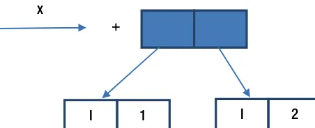
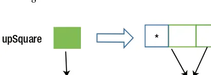
The Cloud and Haskell
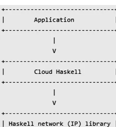
This section discusses the problem of designing distributed processes and implementation processes for cloud environments. Compared with other initial implementations, the aim isn’t to change the API. The API, such as the efforts to combine Erlang-style concurrent and distributed programming in Haskell to provide generic network transport API, libraries intended to send static closures to remote nodes, or a very rich API for distributed programming API, are and represents couple of examples of what we can use in the process of developing applications in Haskell for cloud environments. The real aim is to gain more flexibility in the network layer and transport layer, such as shared memory, IP and HPC interconnects, and configuration (i.e., neighbor discovery startup and tuning network parameters). When designing and implementing software applications with Haskell for the cloud, it’s better to consider both schemes, as shown in Figure 1-1 and Figure 1-2.
Figure 1-1 points outsome dependencies between different modules for the initial startup implementation in Cloud Haskell. The arrows indicate the direction of the dependencies.
Figure 1-1 indicates the initial implementation uses a single specific transport, based on TCP/IP (Haskell network (IP) Library).
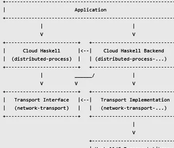
Figure 1-2 shows the various modules that are provided in the new design. We divided a generic system into two layers: the Cloud Haskell layer and the Network Transport layer. Each layer has a back-end package that can be used with different transports.
According to the official documentation (http://haskell-distributed.github.io/wiki/newdesign. html), applications designed and developed with Haskell are encouraged to use the Cloud Haskell Layer.
Complete applications will necessarily depend on a specific Cloud Haskell backend and
would require (hopefully minor) code changes to switch backend. However, libraries of
reusable distributed algorithms could be written that depend only on the Cloud Haskell
package.
The following code example, CountingSomeWords, illustrates how necessary imports are used in a distributed programming environment and how to make them to work with MapReduce.
module CountingSomeWords ( Document
, countingWordsLocally , countingWordsDistributed , __remoteTable
) where
import Control.Distributed.Process
import Control.Distributed.Process.Closure import MapReduce
import MonoDistrMapReduce hiding (__remoteTable) import Prelude hiding (Word)
type DocumentsWithWords = String type SomeWord = String type HowOften = Int
type countWords = Int
countingSomeWords :: MapReduce FilePath DocumentsWithWords SomeWord HowOften HowOften countingSomeWords = MapReduce {
aMap = const (map (, 1) . words) , aReduce = const sum
}
countingWordsLocally :: Map FilePath DocumentsWithWords -> Map SomeWord HowOften countingWordsLocally = localMapReduce countWords
countingSomeWords_ :: () -> MapReduce FilePath DocumentsWithWords SomeWord HowOften HowOften countingSomeWords_ () = countingSomeWords
remotable ['countWords_]
countingWordsDistributed :: [NodeId] -> Map FilePath DocumentsWithWords -> Process (Map SomeWord HowOften)
countingWordsDistributed = distrMapReduce ($(mkClosure 'countWords_) ())
The next example will show how to use one of the most important characteristic of cloud computing within Haskell.
module MapReduce
( -- * Map-reduce skeleton and implementation MapReduce(..)
, localMapReduce
-- * Map-reduce algorithmic components , reducePerKey
, groupByKey
-- * Re-exports from Data.Map , Map
import Data.Typeable (Typeable) import Data.Map (Map)
import qualified Data.Map as Map (mapWithKey, fromListWith, toList) import Control.Arrow (second)
-- | MapReduce skeleton
data MapReduce k1 v1 k2 v2 v3 = MapReduce { mrMap :: k1 -> v1 -> [(k2, v2)] , mrReduce :: k2 -> [v2] -> v3 } deriving (Typeable)
-- | Local (non-distributed) implementation of the map-reduce algorithm
---- This can be regarded as the specification of map-reduce; see -- /Google's MapReduce Programming Model---Revisited/ by Ralf Laemmel -- (<http://userpages.uni-koblenz.de/~laemmel/MapReduce/>).
localMapReduce :: forall k1 k2 v1 v2 v3. Ord k2 => MapReduce k1 v1 k2 v2 v3
-> Map k1 v1 -> Map k2 v3
localMapReduce mr = reducePerKey mr . groupByKey . mapPerKey mr
reducePerKey :: MapReduce k1 v1 k2 v2 v3 -> Map k2 [v2] -> Map k2 v3 reducePerKey mr = Map.mapWithKey (mrReduce mr)
groupByKey :: Ord k2 => [(k2, v2)] -> Map k2 [v2] groupByKey = Map.fromListWith (++) . map (second return)
mapPerKey :: MapReduce k1 v1 k2 v2 v3 -> Map k1 v1 -> [(k2, v2)] mapPerKey mr = concatMap (uncurry (mrMap mr)) . Map.toList
Book Structure
This book has two parts.• Part I is covers eight chapters on the basics of Haskell, including what you need know to develop and move applications in cloud computing and big data environments. • Chapter 1 outlines the most important goals of this book and it guides you
through the entire structure of the book.
• Chapter 2 presents medium-advanced examples of source code that help you understand the difference between creating a software application for local use and a software application used for a cloud-computing environment.
• Chapter 3 brings all the elements for developing software applications using parallelism concurrent techniques. Threads, distributed programming, and EVAL monad for parallelism represent the most important topics.
• Chapter 5 focuses on the importance of using exceptions thrown by different situations of using a monad in order to integrate I/O operations within a purely functional context.
• Chapter 6 covers the importance of cancellation conditions as a major component for developing an application using parallelism.
• Chapter 7 discusses some powerful tools for resolving important issues that could appear in the process of developing distributed applications. These problems include race conditions due to forgotten locks, deadlocks, corruption, and lost wakeups.
• Chapter 8 covers debugging, which plays an important role in the process of developing and updating software applications. Sometimes the debugging process is problematic because Haskell does not have a good debugger for advanced software applications. Some modern techniques that could be used in debugging process are discussed.
• Part 2 is focused on developing advanced software applications using big data and cloud computing environments.
• Chapter 9 covers the most important methods for processes and messages, and techniques used for matching messages. The section will present a domain-specific language for developing programs for a distributed computing environment.
• Chapter 10 covers the most comprehensive techniques and methods for calling and using big data in Haskell by providing case studies and examples of different tasks.
• Chapter 11 goes through concurrency design patterns with the goal to understand how to use them for applications based on big data.
• Chapter 12 presents the steps necessary for designing large-scale programs in such a manner that there are no issues when ported in a big data or cloud environment.
• Chapter 13 looks at Hadoop algorithms and finds the most suitable
environment for running different data sets of varying sizes. The experiments in this chapter are executed on a multicore shared memory machine.
• Chapter 14 covers the necessary tools and methods for obtaining an interactive debugger.
• Chapter 15 presents MapReduce for cloud computing and big data, together with all the elements that can be used for developing professional applications based on data sets and for creating an efficient portability environment. • Chapter 16 offers original ideas for serving applications on data mining,
web ranking, analysis of different graphs, and so on. Elements for improving efficiency by creating and developing caching mechanisms are provided. • Chapter 17 presents case studies that demonstrate the running process on
Summary
This chapter introduced the main ideas behind cloud for Haskell, such as
• the main concepts behind developing Haskell applications for cloud computing environments.
• dependencies and how they are used to gain the greatest performance. • designing modules and setting the new layers necessary for every application
developed with Haskell for the cloud.
CHAPTER 2
Programming with Haskell
Haskell represents a purely functional programming language that provides many advantages and the latest innovations in the design of programming languages. The most recent standard of Haskell is Haskell 2010; but in May 2016, the Haskell community started working on the next version, Haskell 2020.
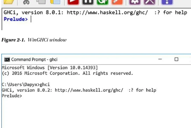
The Haskell platform is available for download at https://www.haskell.org/platform/, where there are other versions of installers and an installation guide. After downloading of the appropriate version, just follow the steps. In this book, we will use version 8.0.1.
This chapter focuses on some of the basic elements that you need to understand before continuing to the next chapters. The information is intended for the users and programmers who already have some experience in Haskell programming.
Functional vs. Object-Oriented Programming
Before starting programming with Haskell, it is important to understand the principles of functional programming (FP), and the similarities and the differences between it and object-oriented programming (OOP). We assume that you have (at least) a basic knowledge of object-oriented programming.
The purpose of OOP and FP is to create programs that are easy to understand, flexible, and have no bugs; but each paradigm has its own approach.
Broadly, the similarities between the two programming paradigms are in the levels of expressive power and the capabilities of encapsulating programs into more compact pieces that could be (re)combined. The main difference is the connection between data and the way operations are applied on that data.
The most important principle of OOP is that the data and the operations applied on that data are closely linked: an object contains its own data and the specific implementation of the operations on the owned data. Thereby, the main model to be abstracted is the data itself. OOP allows you to compose new objects, but also to extend the existing classes through the addition of new methods.
Language Basics
This section discusses Haskell programming basics, but first you need to understand the components of a Haskell program.
• The most important level of a Haskell program is a set of modules that allow you to control namespaces and reuse software in big programs.
• At the top of a module, there are the declarations that define different elements (for example, values, or data types).
• The next level is represented by expressions, which is static and designates a value. These are the most important elements of Haskell programming.
• The last level is represented by the lexical structure, which catches the concrete frame of Haskell programs in the text files.
A value is evaluated by an expression, which has a static type. The type system permits defining new data types and more types of polymorphism (parametric or ad hoc).
In Haskell, there are several categories of names. • Values. The names for variables and constructors
• Elements associated with the type system. The names for type constructors, type variables, and type classes
• Modules. The names for modules
You need to pay attention when naming variables and type variables. These names represent identifiers, which should start with a lowercase letter or an underscore. Other names should begin with an uppercase letter.
As in every programming language, comments are allowed. To comment on a single line, use -- before the comment. A multiline comment begins with {- and ends with -}. The following are examples.
-- This is a single line comment. {- This is
a multi-line commnet. -}
Arithmetic
Now that you know a few things about Haskell language programming, let’s do some arithmetic. The following are examples of using the arithmetic operators +, -, *, and /.
Prelude> 5 + 3 8
Prelude> 175 - 23 152
Prelude> 55 * 256 14080
Prelude> 351 / 3 117.0
Prelude> 5 + 3 8
Prelude> 175 - 23 152
Prelude> 55 * 256 14080
Prelude> 351 / 3 117.0
Figure 2-1. WinGHCi window
You can combine these operators by using parenthesis. If you want to operate with a negative number, you should use the parenthesis—for example 5 * (-3); otherwise, you will get an error message. Also, there are mathematical functions such sqrt, abs, min, max, and succ.
Prelude> 133 * 18 + 5 2399
Prelude> 133 * (18 + 5) 3059
Prelude> 374 / (20 - 31) -34.0
Prelude> 3 + sqrt(9) 6.0
Prelude> abs(25-100) 75
Boolean algebra is permitted. True and False represent the two Boolean values. As in other
programming languages, && represent the Boolean and, || represents the Boolean or, and the keyword not represents negation. Also, you can test equality by using the == (equal) or /= (not equal) operators. Prelude> True && False
False
Prelude> False || True True
Prelude> not True False
Prelude> (True || False) && (not True) False
Prelude> 100 == 100 True
Prelude> 100 /= 100 False
■
Note
The
Trueand
Falsevalues begin with an uppercase letter.
When you use arithmetic operators or Boolean operators, the left side and the right side of the operator should have the same type; otherwise, you will get an error message.
Prelude> 2 + 2 4
Prelude> "xy" == "xy" True
Prelude> 2 + "xyz"
<interactive>:26:1: error:
• No instance for (Num [Char]) arising from a use of '+' • In the expression: 2 + "xyz"
In an equation for ‘it’: it = 2 + "xyz" Prelude> True && 5
<interactive>:29:9: error:
• In the second argument of '(&&)', namely '5' In the expression: True && 5
In an equation for 'it': it = True && 5 Prelude> 3 == "xy"
<interactive>:30:1: error:
• No instance for (Num [Char]) arising from the literal '3' • In the first argument of '(==)', namely '3'
In the expression: 3 == "xy"
In an equation for 'it': it = 3 == "xy"
In the preceding example, the + operator also expects a number on the right side, and the && operator expects a Boolean value on the right side. The equality can be verified only between two items of the same type. The example tests the equality between two strings, which is successful, and between a number and a string, which are different types, so there is an error message. Still, there are some exceptions when you operate with items of different types. This is when implicit conversion occurs. For example, addition using an integer value and a point value is allowed because the integer can be converted to a floating-point number. The following is an example.
Prelude> 3 + 2.5 5.5
Pairs, Triples, and Much More
If you want to set a specific value or expression to a variable, use the keyword let. You do not need to declare the variable before setting a value. In Haskell, once you set a value to a variable, you cannot change that value in the same program. It is similar to a problem in mathematics—a variable cannot change its value in the same problem. The variables in Haskell are immutable. The following advanced example shows that if you set two values to a variable, you will get an error.
Prelude> let x = 4 Prelude> x
4
Prelude> let y = "abc" Prelude> y
"abc"
Tuples are useful when you know the number of values to be combined. Tuples are marked by
parenthesis. Its elements are separated by commas; they are not homogenous and they can contain different types.
Prelude> let pair = (2, "orange") Prelude> pair
As you can see in the preceding example, our tuple is a pair with two elements of different types: a number and a string. Tuples are inflexible, because every tuple with its own size and types actually represents a type itself. Thus, general functions for tuples cannot be written. For example, if you want to add an element to a tuple, you should write a function for a tuple with two elements, a function for a tuple with three elements, and so on. You can make comparisons between tuples only if their components can be compared.
Prelude> let fstTuple = ("apple", 2, True) Prelude> let sndTuple = ("orange", 3, True) Prelude> fstTuple == sndTuple
False
Prelude> let trdTuple = ("green", False) Prelude> fstTuple == trdTuple
<interactive>:53:13: error:
• Couldn't match expected type ‘([Char], Integer, Bool)’ with actual type ‘([Char], Bool)’
• In the second argument of ‘(==)’, namely ‘trdTuple’ In the expression: fstTuple == trdTuple
In an equation for ‘it’: it = fstTuple == trdTuple
There are two important functions, which are applied on a particular type of tuples, namely the pair: fst and snd. Intuitively, fst returns the first element of the pair and snd returns the second element of the pair. In Haskell, you call a function by writing its name, followed by parameters divided by spaces.
Prelude> fst trdTuple "green"
Prelude> snd trdTuple False
Prelude> fst (5, True) 5
Lists
Lists are similar to tuples. The main difference between them is that the lists are homogenous data structures; thus, all elements are of the same type. For example, you can have a list of integers, or a list of characters, but you cannot mix them in the same list. Lists are marked by brackets, and the elements are separated by commas. The strings are a list of characters, so the "Haskell" string is actually the list ['H', 'a', 's', 'k', 'e', 'l', 'l']. You can apply different functions on lists. Thus, because strings are lists of characters, you can apply many functions on them.
Prelude> [1, 2, 3] ++ [4, 5] [1,2,3,4,5]
The ++ represents the concatenation of the left-side list with the right-side list (with elements of the same type). When two lists are concatenated, the left-side list is traversed entirely, and the elements of the right-side list are added at the end of the first list. This could take a while if the left-side list has many elements. Intuitively, adding an element to the beginning of a list is much faster. To add an element at the beginning of the list, use the cons operator ( : ).
Prelude> 1:[2,3,4] [1,2,3,4]
Prelude> 'A':" flower" "A flower"
■
Note
In the second example, the character is between single quotes, and the string is between double
quotes.
If you want to extract an element on a particular index, use !!. Pay attention to the chosen index: if it is greater than the number of elements, or if it is negative, you will get an error message. The first index in a list is 0. A list can contain other lists, with the following rule: the lists can have different sizes, but they cannot contain different types.
Prelude> [2,4,6,8,10] !! 4 10
Prelude> [2,4,6,8,10] !! 6
*** Exception: Prelude.!!: index too large Prelude> [2,4,6,8,10] !! -5
<interactive>:64:1: error: Precedence parsing error
cannot mix ‘!!’ [infixl 9] and prefix `-' [infixl 6] in the same infix expression Prelude> [[1,2], [3], [4,5,6]]
[[1,2],[3],[4,5,6]]
Lists can be compared if they contain elements that can be compared. The first element of the left-side list is compared with the first element of the right-side list. If they are equal, then the second elements are compared, and so on.
Prelude> [1,2,3] < [5,6,7] True
Prelude> [1,2] < [-1,6,7] False
There are many useful functions in lists, such as length,head,tail,init,last,maximum,minimum,sum, product,reverse,take,drop,elem,null, and much more. Figure 2-3 is an intuitive representation of the results of the functions head,tail,init, and last.
Prelude> length [1,2,3,4,5] 5
Prelude> head [1,2,3,4,5] 1
Prelude> tail [1,2,3,4,5] [2,3,4,5]
Prelude> init [1,2,3,4,5] [1,2,3,4]
Prelude> last [1,2,3,4,5] 5
Prelude> minimum [1,2,3,4,5] 1
Prelude> maximum [1,2,3,4,5] 5
Prelude> reverse [1,2,3,4,5] [5,4,3,2,1]
Prelude> sum [1,2,3,4,5] 15
Prelude> drop 3 [1,2,3,4,5] [4,5]
Prelude> take 2 [1,2,3,4,5] [1,2]
Prelude> elem 6 [1,2,3,4,5] False
■
Note
The empty list is
[]. It is widely used in almost all recursive functions that work with lists. Note that
[]and
[[]]are distinct things, because the first is an empty list and the second is a non-empty list with one
empty list as an element.
init
last
head
tail
Source Code Files
In practice, source code is not written in GHCi; instead, source code files are used. Haskell source code files have the extension .hs. Let’s suppose that you have a file named Main.hs with the following source code. main = print (fibo 5)
fibo 0 = 1 fibo 1 = 1
fibo n = fibo (n-1) + fibo (n-2)
This source code represents a function that computes the Fibonacci number on a specific index. For the moment, take the function as it is; we will explain it in the next subsection. Let’s recall how to compute the Fibonacci numbers: F(0) = 0, F(1) = 1, F(n) = F(n-1) + F(n-2), where n > 1.
Now, let’s return to the source code files. The file could be saved anywhere, but if the work directory is different from the current directory, you need to change it to that directory in GHCi, using the :cd command, as follows.
Prelude> :cd C:\Users
To load a file into GHCi, use the :load command. Prelude> :load Main
After loading the module, you can observe that the prompt was changed into *Main> to indicate that the current context for expression is the Main module. Now, you can write expressions that include functions defined in Main.hs.
*Main> fibo 17 2584
When loading a module, GHC discovers the file name, which contains, for example, a module M, by looking for the file M.hs or M.lhs. Thus, usually, the name of a module should be the same as the file; otherwise, GHCi will not find it. Still, there is an exception: when you use the :load command for loading a file, or when it is specified invoking ghci, you can provide the file name instead of a module name. The specified file will be loaded if it exists, and it could comprise any number of modules. If you are trying to use multiple modules in a single file, you will get errors and consider it a bug. This is good, if there are more modules with the same M name, in the same directory; you cannot call them all M.hs.
If you forget the path where you saved a source code file, you can find it, as follows. ghci -idir1:...:dirn
If you make changes in the current source code file, you need to recompile it. The command for recompilation is :reload, followed by the name of the file.
Functions
You haven’t used the return keyword. This is because Haskell does not have a return keyword; a function represents a single expression, not a succession of statements. The outcome of the function is the worth of the expression. Still, Haskell has a function called return, but it has a different meaning than in other programming languages.
Let's write a simple function that computes a power. Prelude> pow a b = a ^ b
Prelude> pow 2 10 1024
A function has a type, which could be discovered using the :type command. Prelude> :type pow
pow :: (Num a, Integral b) => a -> b -> a
As secondary effect, a dependence on the global state and the comportment of a function is introduced. For example, let’s think about a function that works with a global parameter, without changing its value and returning it. When a piece of code changes the value of the variable, it affects the function in a particular way, which has a secondary effect; although our function does not change the value of the global variable, which is treated as a constant. If a variable is mentioned out of scope, the value of the variable is obtained when the function is defined.
The secondary effects are usually invisible outcomes for functions. In Haskell, the functions do not have secondary effects, because they are depending only on explicit arguments. These functions are called pure. A function with side effects is called impure.
Prelude> :type writeFile
writeFile :: FilePath -> String -> IO ()
The Haskell type system does not allow combining pure and impure code.
if-else
As in other programming languages, Haskell also has the if-else statement. Its syntax is very simple. Let’s write a function that returns the maximum between two values.
Prelude> maximum a b = if a > b then a else b maximum :: Ord t => t -> t -> t
Prelude> maximum 5 6 6
An important aspect of Haskell is indentation. You need to pay attention to how you organize your code. For example, if you write the maximum function in an .hs file, then it should look like the following.
maximum a b = if a > b
then a else b
The if-else statement has three elements:
• A predicate, which represents the Bool expression which follows the if keyword • The then keyword, which is followed by an expression, and evaluated if the
expression that follows the if statement is True
• The else keyword, which is followed by another expression, and evaluated if the expression that follows the if statement is False
The two expressions that follow then and else are called branches. They should be the same type; otherwise, it will be cancelled by the compiler/interpreter. The following example is wrong because 10 and abc have different types.
If expression then 10 Else "abc"
In Haskell, the if-else statement without an else statement is not allowed, because it is a programming language based on expressions.
RECURSION
The recursion is very important because many functions are recursive, and it represents a manner in
which a function is called by itself. Let’s remember a previous example: the function that computes
Fibonacci numbers. For example, if you call
fibo(4) = fibo(3) + fibo(2) = (fibo(2) + fibo(1)) + (fibo(1) + fibo(0)) = ((fibo(1) + fibo(0)) + 1) + (1 + 0) = ((1 + 0) + 1) + 1 = (1 + 1) + 1 = 2 + 1 = 3
As you can see,
fibo(4)calls
fibo(3)and
fibo(2), and so on. The elements of the function that are
not defined recursively are called edge condition. They are extremely important because they represent
the conditions needed to escape from recursion.
The recursion represents one of the base elements of Haskell, because it shows us what something is,
rather than how it is computed. Also, it replaces
forand
whileloops.
Types
Simple vs. Polymorphic Types
A simple value is a value that has only one type. This is discussed more about types in the “Data Types” section.
A polymorphic value is that value which could have multiple types. It is a very useful and used feature of Haskell. There two main types of polymorphism: parametric and ad hoc.
Parametric Polymorphism
Parametric polymorphism occurs if the variable has more than one type, such that the its value could have any type resulted from replacing the variable with explicit types. This means that there are no constraints regarding type variables. The simplest and the easiest example is the identity function.
Identity :: a -> a
The a can be replaced with any type, whether it is a simple type, such as Int, Double, Char, or a list, for example. So, for a, there is no constraint regarding the type.
The value of a parametrically polymorphic type has no knowledge of type variables without constraints, so it should act in the same way regardless of its type. This fact is known as parametricity, and it is very useful, even if it is limiting.
Ad hoc Polymorphism
Ad hoc polymorphism occurs when a variable chooses its type according to its behavior at a particular moment, because it is an implementation for every type. A simple example is the + function. The compiler should know if it is used to add integers, or two floating-point numbers.
In Haskell, ambiguity is avoided through the system of type classes or class instances. For example, to compare two objects, you need to specify how the == operator behaves. In Haskell, the overloading is extended to values; for example, a lowerLimit variable could have different values according to its use. If it refers to an Int, its value cloud is –2147483648, and if it refers to Char, its value could be '\NUL'.
Type Classes
In Haskell, you identify the following aspects of type: strong, static, and automatically inferred.
The strong type system of Haskell assures the fact that a program does not contain errors obtained from expressions without a meaning for compiler.
When a program is compiled, the compiler knows the value of every type before the code is executed. This is assured by the static type system. Also, when you write expressions of different types, you will get an error message. By combining the strong type and the static type, the type errors will not occur at runtime. Prelude> 2 + "5"
<interactive>:28:1: error:
• No instance for (Num [Char]) arising from a use of '+' • In the expression: 2 + "5"
At compilation, each expression’s type is known. If you write an addition symbol between a number and a Boolean value, you will get an error message. In Haskell, each thing has a type. A benefit of Haskell is that it has the type inference, through which the type is implicitly inferred. So, if you write a number, you do not need to specify that it is a number.
Strong and static types bring security, while inference makes Haskell concise, so you have a safe and an expressive programming language.
Function Types
In Haskell, the functions have types. When you write functions, you can give them an explicit declaration, a fact that is helpful when you deal with complex functions. If you want to declare a function, you proceed as follows.
getMax :: [Int] -> Int
The meaning is intuitive. In the preceding example, the getMax function returns the maximum value from a list of integers. The :: symbol is followed by the domain of the definition of the function, and the -> shows the type of the result.
If you have a function with more parameters, you proceed as follows. addition :: Int -> Int -> Int
Here, you have the addition function, which computes the sum of the two integers. The first two Ints show the type of the parameters, and they are divided by the -> symbol, and the last Int shows the result type.
It is recommended that functions be written with the explicit declaration; but if you are not sure about that, you can just write the function, and then check its type using the :t or :type commands.
Data Types
The following are some basic data types.
• Int: Integer numbers, which are signed and have fixed width. The range of values is not actually fixed; it depends on the system (32/64 bits), but Haskell assures that an Int is larger than 28 bits.
• Integer: Integer numbers with unbounded dimensions. The Integer type consumes more space and is less performant than Int, but it brings more dependably correct answers. In practice, it is used less than Int.
• Double: Floating-point numbers. Usually, the double value is represented in 64 bits, using the natural floating-point representation of the system.
• Char: Unicode character.
• Bool: A value from Boolean algebra. There are only two possible values: True and False.
If you want to check the type of value or an expression, you simply use the :t command, followed by the value or expression, as follows.
Prelude> :t 5.3
5.3 :: Fractional t => t Prelude> :t "abcd" "abcd" :: [Char] Prelude> :t (5 < 2) (5 < 2) :: Bool
Input/Output (IO) Mechanisms
GHCi accomplishes more things than evaluating straightforward expressions. When an expression has the type IO a, for some a, GHCi is executing it like an IO computation. Basically, a value which has type (IO a) represents an action that when it is executed, its result has type a.
Prelude> length "Haskell" 7
Prelude> 100/2 50.0
When an expression’s type is general, it is instantiated to IO a. Prelude> return True
True
The result of an expression’s evaluation is printed if • It represents an instance of Show
• Its type is not ()
In order to understand the following example, it is necessary to understand do notation. By using do, the notation (instruction) represents an alternative to the monad syntax.
The following example implies IO and you refer to the computation’s values as actions. It’s important to mention that do is applied with success with any monad.
The >> operator works in the same way as in do notation. Let’s consider the following example, which is formed from a chain of different actions.
putStr "How" >> putStr " " >>
putStr "is with programming in Haskell?" >> putStr "\n"
The following example can be rewritten using do notation. do putStr "How"
putStr " "
As you can see, the sequence of instructions almost matches in any imperative language. In Haskell, you can connect any actions if all of them are in the same monad. In the context of the IO monad, the actions that you are implementing could include writing to a file, opening a network connection, and so forth.
The following is a step-by-step translation in Haskell code. do action1
action 2 action 3
becomes action1 >> do action2 action3
and so on, until the do block is empty.
Besides expressions, GHCi takes also statements, but they must be in the IO monad. Thus, a name could be bounded to values or a function for further use in different expressions or statements. The syntax of a statement is the same as the syntax of do expressions.
Prelude> x <- return "abc" Prelude> print x
"abc"
The preceding statement, x<-return "abc" could be “translated,” so execute return “abc” and link the outcome to variable x. Later, the variable could be used in other statements; for example, for printing.
When -fprint-bind-result is enabled, the outcome of a statement is typed if
• the statement does not represent a binding, or it is a binding to a single variable (v <- e).
• the type of the variable does not represent polymorphism, or (), but it represents a Show instance.
The binding could also be done using the let statement. Prelude> let y = 10
Prelude> y 10
A characteristic of the monadic bind is that it is strict; namely, the expression e is evaluated. When using let, the expression is not instantly evaluated.
Prelude> let z = error "This is an error message." Prelude> print z
*** Exception: This is an error message. CallStack (from HasCallStack):
error, called at <interactive>:18:9 in interactive:Ghci8
Another important thing is that you can write functions directly at the prompt. Prelude> f x a b = a*x + b
Nevertheless, this will be a little awkward when you are dealing with complex functions, because the implementation of the function should be on a single line.
Prelude> f a | a == 0 = 0 | a < 0 = - a | a > 0 = a Prelude> f 100
100
Prelude> f (-324) 324
Prelude> f 0 0
But Haskell comes with a solution. The implementation could be divided into multiple lines, using the :{ and :} commands.
Prelude> :{ Prelude| f a
Prelude| | a == 0 = 0 Prelude| | a < 0 = -a Prelude| | a > 0 = a Prelude| :}
If an exception occurs while evaluating or executing statements, they are caught and their message is typed, as you have seen in previous examples.
The temporary binds can be used the next time you load or reload a file, because they will be missed after (re)loading, but can be used after the :module: command (discussed in the next section) when it goes to another location. If you need to know all of the binds, you can use the following command.
Prelude> :show bindings x :: [Char] = "abc" y :: Num t => t = _ it :: Num t => t = _ z :: a = _
If +t is enabled, you can find every variable’s type. Prelude> :set +t
Prelude> let (x:xs) = [1..] x :: Integer
xs :: [Integer]
There is another possibility that GHCi identifies when a statement is not terminated, and permits writing on multiple lines. It is enabled by the :set +m command. The last line is empty to mark the end of multiple line statement.
If you want to bind values to more variables in the same let command, you should proceed as follows: Prelude> :set +m
Prelude> let a = 154887 Prelude| b = 547 Prelude|
For multiple line statements, you can use do. The individual statements are separated by semicolons. The right brace marks the end of the multiline statement.
Prelude> do { Prelude| print b Prelude| ;print b^ 2 Prelude| }
547 299209 Prelude>
The multiple-line statements could be interrupted as follows. Prelude> do
Prelude| print a Prelude| ^C Prelude>
Haskell has a special variable, called it, which receives the value of an expression typed in GHCi (of course, the expression should not be a binding statement).
Prelude> 2*3 6
Prelude> it+5 11
You need to remember that an expression must have a type, instantiated from Show; otherwise, you will get an error message.
Prelude> head
<interactive>:14:1: error:
• No instance for (Show ([a0] -> a0)) arising from a use of 'print' (maybe you haven't applied a function to enough arguments?) • In a stmt of an interactive GHCi command: print it
Haskell permits the use of command-line arguments through the getArgs function, which is passed to the main using the :main command.
Prelude> main = System.Environment.getArgs >>= print Prelude> :main abc xyz
["abc","xyz"]
Prelude> :main abc "xyz pq" ["abc","xyz pq"]
Prelude> :main ["abc", " xyz pq "] ["abc","xyz pq"]
Any function could be called using -main-is or the :run commands. Prelude> abc = putStrLn "abc" >> System.Environment.getArgs >>= print Prelude> xyc = putStrLn "xyz" >> System.Environment.getArgs >>= print Prelude> :set -main-is abc
Prelude> :main abc "xyz pq" abc
["abc","xyz pq"]
Prelude> :run xyz ["abc","xyz pq"] xyz
["abc","xyz pq"]
Modules
This section introduces the notations and information necessary for understanding the rest of the book. It’s important to acknowledge the fact that a module in Haskell serve in two directions with a specific purpose: controlling namespaces and creating abstract data types. This aspect is very important in understanding complex applications that are developed in a cloud and big data environment.
If you are looking at a module from a technical perspective, a module is a very big declaration that starts with module keyword. Consider the following example, which presents a module called Tree.
module Tree (Tree(Leaf, Branch), fringe) where
data Tree a = Leaf a | Branch (Tree a) (Tree a)
fringe :: Tree a -> [a] fringe (Leaf x) = [x]
fringe (Branch left right) = fringe left ++ fringe right
The following example is presented from official documentation available at https://www.haskell. org/tutorial/modules.html, which has the best explanation. It can be used as a prototype for different tasks that can be implemented into a distributed environment. An important operation in the preceding example is the ++ infix operator, which concatenate the two lists, left and right. In order for the Tree module to be imported into another module, follow this code snippet.
module Main (main) where
import Tree (Tree((Leaf, Branch), fringe)
The various items that are imported into and exported outside of the module are called entities. Observe the explicit import list in the declaration of the import. If you omit this, it would cause all the entities that are exported from Tree to be imported.
:load/:reload
As you already know, the default module of Haskell is Prelude. You can change it by importing another module using the :load command. When it is appended, it automatically imports into the scope corresponding to the last loaded module. To be certain that GHCi imports the interpreted version of a module, you can add an asterisk when you load it, such as :load *modulename.
Prelude> :load Main.hs
Compiling Main ( Main.hs, interpreted ) *Main>
Now, you can use expressions that involve elements from the loaded module. The star that accompanies the name of the module shows that the module represents the full top-level scope of the expressions from the prompt. In the absence of the asterisk, only the module’s exports are observable.
:module
The :module command also permits scope manipulation. If the module keyword is accompanied by +, then the modules are added; if it is accompanied by -, then the modules are removed. If there is no + or -, the actual scope is substituted by the modules after the :module command.
The use of module brings more benefits than using the import command. The main facilities are • the full top-level of a scope is opened through the * operator.
• the unneeded modules can be removed.
:import
The :import command is used to add modules. Prelude> import Data.Char
Prelude> toUpper 'a' 'A'
To see all imported modules, use the :show imports command. Prelude> import System.IO
Prelude> :show imports import Prelude -- implicit import Data.Char
import System.IO
As you have seen, there are two ways to get a module in the scope: by using :module/import or by using :load/:reload. Still, there are significant differences between the two approaches in the collection of the modules.
• The collection of modules that are loaded. changed using :load/:reload and viewed using :show modules.
• The collection of modules in the scope at the prompt. changed using :module/import, and instantaneous after :load/:reload, and viewed using :show imports.
A module can be added into the scope (through :module/import) if • the module is loaded.
• the module belongs to a package known by GHCi. In any other cases, it will be an error message.
Operators Used as Sections and Infix
In Haskell, there are two types of notations used for function calling: prefix notation and infix notation. Usually, prefix notation is used: the name of the function, followed by the arguments. The infix notation is where the name of the function stands between its arguments. Note that the infix notation can be used for functions with two parameters. If the function has more than two parameters, then the infix notation becomes inconvenient and difficult to follow.
The best-known infix functions are operators. As you well know, the arithmetic operators take two arguments, so they are by default infix. However, if you begin the line with an arithmetic operator in parenthesis, followed by the two arguments, then it becomes a prefix function.
Prelude> (+) 4 5 9
Prelude> (*) 10 10 100
Anyway, there is a way to use infix notation for an ordinary function. This is done by putting the name of the function between the ` symbol, as follows.
Prelude> let concatPrint x y = putStrLn $ (++) x y Prelude> concatPrint "a" "b"
ab
Prelude> "a" `concatPrint` "b" ab
There is a particular language structure for an incomplete application on infix operators. Broadly, when you use an operator, it behaves like a function that receives one of the arguments, and the other is put in the place of the misplaced side of the operator.
Sectioning a function is very useful because it allows you to write a function, without giving a particular name to that function; for example:
• (1+): the function which increments by one a value • (2*): the function which doubles a value
• ('\t':): the “tab” function
The minus operator cannot make a right section, since it would be deciphered as unary invalidation in the Haskell language. The Prelude capacity “subtract” is accommodated this reason.
Local Declarations
In Haskell, local declarations can be used. This is done by using the let keyword, which binds a particular value to a variable; for example:
Prelude> let a = -5 + 1 in a + 10 6
This is equivalent to {
int a = -5 + 1; ... a + 10 ... ; }
In Haskell, the variable receives a value that cannot be changed.
Partial Application
When a function is called with some arguments missing, you actually obtain another function. This can be seen as something like “underloading,” but the specific term is partial application. For example, let’s think about the power function. It takes two arguments: namely, the base and the exponent. If you have a program in which only the irrational number e is used as a base, you could define a new function that takes one argument— namely, the exponent, as follows.
Prelude> powE x = (exp 1) ^ x
powE :: (Integral b, Floating a) => b -> a Prelude> powE 5
148.41315910257657
This is very useful when you have complex functions with many parameters, but most of the time, you do not use all parameters.


![[Bookflare net] Next Generation Big Data A Practical Guide to Apache Kudu, Impala, and Spark pdf pdf](data:image/gif;base64,R0lGODlhAQABAIAAAP///wAAACH5BAEAAAAALAAAAAABAAEAAAICRAEAOw==)