A Continuous Topography Approach for Agent Based Traffic Simulation, Lane Changing Model

A Continuous Topography Approach for Agent Based

Traffic Simulation,

Lane Changing Model*

Ade Jamal

Department of Informatics, University Al-Azhar Indonesia Jl. Sisingamangaraja, Kebayoran Baru, Jakarta 12110

E-mail: adja@uai.ac.id

Abstract  Traffic simulation has been being an

interesting research subject for transport engineer and scientist, mathematicians and informatics scientist for different point of view. Transport scientists study the traffic complexity and behaviour of traffic participants by using statistical experiment or simulation. The earlier approach was based on macroscopic model deducted from hydrodynamics kinematic wave analogy. Later on the microscopic model was introduced first by invoking cellular automata and then agent based model takes important role in the traffic simulation world. Most of microscopic model are based on a multi-grid element topography model which is a natural environment of cellular automata. Just recently a software engineer started an ambitious work to develop a multipurpose framework for complex traffic simulation. The ingenious idea is to replace the traditional grid based element topography with a continuous two dimensional one from which a region of traffic road or street is built up. Traffic participant is modelled as agent whose physical properties such as its coordinate position, speed, and direction are governed by the kinematic Newtonian law. This article will present this new concept and show how the simple movement of lane changing model that is very well known from the beginning era of traffic simulation become a quite complex movement in the new continuous topography

Keywords - traffic simulation; agent based model;

lane changing; geometry analysis



This paper has been presented in The 1st International Conference on Computer Science, Electronics and Instrumentation, Yogyakarta, 12-13 November 2012

I. INTRODUCTION

imulation of traffic has been attracting many researchers from many different fields, especially in the field of transport and computer science. For transport engineers and scientists, where traffic problem is their specific domain, researches on traffic simulation is more focus on traffic theory such as traffic complexity and behaviour of traffic users, and the use of traffic simulator to solve the various problems related to the traffic. In the earlier period, traffic simulation was modelled by transport scientist based on traffic theory according to hydrodynamic concept, where the traffic flow is described as continuum. This model approach is then called macroscopic model as opposed to the microscopic model which later getting more popular since the influence of computer technology is a must in the traffic simulation. In the microscopic traffic simulation model, the trajectory of every single vehicle is calculated as function of time. By integrating and accordingly averaging of all microscopic traffic parameter of each vehicle, one can redeem to the macroscopic traffic characteristics [1].

In the earlier phase of microscopic model, the traffic simulation was modelled as single lane, i.e. the system consists of a one dimensional grid with periodic boundary. Two basic models are very often used i.e. car-following model [1, 2, 3, and 4] and lane-changing model [1] in the microscopic single lane model. A mathematicians and physician scientist [5] has incorporated cellular automata (CA) to introduce a two lane model consisting of two parallel single lane models with periodic boundary conditions and additional rules defining the exchange of vehicles between the lanes. In this CA multi-lane model, vehicle’s movement takes place in two steps, first completely sideway and then forward. The CA mode has received many

interests during 90’s as it can run large and

relatively complex traffic simulations such urban traffic with only comparatively low computational resources [6].

While mathematicians successfully invoked CA for simulation model, computer scientist proposed (multi)-agent based modelling (ABM) for the traffic simulation [7]. ABM gains its popularity in the last decade [8, 9]. Dijkstra [10] has combined CA and ABM to model pedestrian movement using a regular grid based topography model. While in the single or multi-lane microscopic model, traffic participant can only move forward or lateral only in every (sub)-step, in the regular grid structure topography, any traffic participant can move in any direction as long as no obstacles blocking the movement.

More recently, Ulf Lotzmann in [11, 12] has proposed a very different approach where ABM based microscopic traffic simulation uses a continuous topography model instead of grid based topographical model. The cellular automata is replaced by a finite automata (finite state machine) for modelling dynamic simulation process. The objective of this latest study is development of framework for multipurpose simulation of complex traffic.

The present study is inspired by Ulf Lotzmann’s

innovation, especially the application of continuous environment for precise and realistic design of crowded urban traffic such with various types of traffic users. In this initial stage of work, we will focus on the lane changing movement.

II. NEW TRAFFIC SIMULATION APPROACH

1.1 Agent Based Model

By definition, an agent is an autonomous entity that cannot be controlled by external interference and it can interact with other agents and environment by means of a specified communication system. Agent can perceive events within its environment and can react accordingly. In any ABM typed traffic simulator, every traffic participant can be identified as agent. Some ABM simulator considers environment also as a passive agent as in [11]. In the present work, the environment is distinguished from agent if it has no ability to interact actively with agents. This kind of environment is modelled as topography that includes road, street, sidewalks,

building and others. However, proactive environmental objects such traffic light could be taken into account as a non-moveable agent.

Fulfilling the requirement above, an ABM typed simulator should have the following components: 1. Agent models representing traffic participants

with their physical attributes and their physical layer represents the real-world physical properties of agents such as position, speed, direction and other parameters attached to the

agent’s physical entity. This is the only layer that

has interface to outside world of agent, whether for the sake dynamic process of simulation or for visualization infrastructure.

How the agent behaves is modelled in the behavioural layers. In [8, 11, and 12] this layer is further divided into two functional layers. The first layer that will interact directly with the physical selection. This intelligent layer is called artificial Intelligent layer in [11, 12]. The strategic layer will first perceive the robotics perception and then will provide an intelligent action to be performed by robotic layer accordingly.

1.3 Topography Model

Topography model represents the environmental elements in the real-world such as road, street, building, and pedestrian sidewalks. In the traditional microscopic model, topography model uses CA to represent only driveable region such freeways, roads and streets. In this CA model

vehicle can only move forward or “unrealistically”

Another limitation of grid based CA model is that the accuracy of detail representation of the real-world depends on the size of each grid element. In the most traffic simulation on the road, grid element size is as big as average vehicle size [4, 5, 6, and 7] or as small as people size for simulation pedestrian movement in [10]. To mix this different size of traffic participants, the grid based model for topography is inefficient [12].

The new approach of topography model is by using continuous two-dimensional space in the topography region. Noted that a topography region is a limited and closed polygon shape area with homogeneous attribute that can be entered by traffic participants than can occupy any place within the region. An important restriction of a region that its attribute must be homogeny will determine the size and the shape of the region.

Using the continuous topography model, the previous limitation of lateral movement and inefficiency of grid size problem is minimized. However, this more flexibility in the continuous regions means mathematical and logical model of movement become more complex than in the grid based model.

Figure 1. Three agent behaviour layer [12]

III.CONTINUOUS TOPOGRAPHY MODEL

Agent movement in the continuous region will involve properties in the physical layer and to some extent the robotic operative behaviour layer. Prior to presenting the agent movement mechanism, these will be briefly described in this section.

3.1 Continuous region

Traffic roads and streets must be built up from a number of continuous regions as an example Fig. 2 shows a traffic crossing road. The small arrow indicates the homogeny formal direction of traffic in the corresponding region. This direction is a guide line to follow but the moving participants in that region are not necessary to follow this precisely. The direction is measured as the angle with respect to the global vertical up direction.

3.2 Agent physical layer and robotic behaviour layer

Physical layer subsumes real properties of agent that represent actual geometry conditions of the traffic participants such as its coordinate position in

(x,y), speed v, direction φ and shape. Some of these

properties are unchanged during the simulation, e.g. shape. However, the most of physical properties will vary as response to the action order from the robotic layer.

This autonomous robot is modelled by applying the Finite State Machine (FSM). In the lieu of object oriented paradigm, a complex FSM can be split up

into some smaller and simpler FSM’s. For instance,

the lane change model is a single simple action in the traditional microscopic model, but it is actually a complex action in the continuous topography model. The lane changing starts with turning or bending to the side boundary of the region, and then followed by lane centring which in turn consisting of two opposite bending movement.

Hence the robotic layer is divided into the following sub layers [12]:

1. Level one represents basic actions which are usually conducted without thinking by humans (e.g. turning the steering wheel). The state activities on this level directly modify the physical agent attributes during the lapse of time. Due to the time-discrete simulation model, the activities are adjusted for the duration of a discrete time step. Furthermore, state activity and transition function are executed at every time step.

2. Level two deals with activities composed of basic actions (e.g. hold the centre of a lane). The state-activities at this level configure the transitions for the level 1 automaton. A possible state transition at level 2 is triggered by the transition functions of level 1.

3. Level three subsumes all required plans for complex activities a human is aware of when executing (e.g. lane change operation). The impact of activities and the mechanism for triggering a transition is analogue to the level 2 automaton. The transition functions for level 3 are provided by the AI strategic behaviour layer.

Each of these sub layers has a communication system namely sensor that perceives data from the environment and then make a perception on these data which in turn will be returned to the associated sub layer. Detail on this sensor and FSM of sub layer level two and three is out of scope this article. This article will present a more detail movement mechanism of complex action, in this case the famous lane changing model. However for the sake of completeness, FSM of basic action from level one is presented in Fig. 3.

Figure 3. FSM for robotic basic action level 1 [12]

There are four basic actions, namely [12]:

1. Idle: the vehicle remains steady in the current state. Speed v and heading direction φ remain constant.

2. Accelerate: the driver accelerates or decelerates the vehicle by accelerating intensity a to the desired speed v.

3. Bend: the driver turns the steering wheel with the angular radius m in order to gain a new

direction α where linear speed v remains constant and the heading direction φ is modified

accordingly.

4. Unsteady bend (accelerate and bend): combination of accelerate and bend where both

linear speed v and the heading direction φ are

modified.

IV.DETAIL MOVEMENT IN THE CONTINUOUS

TOPOGRAPHY MODEL

4.3 Mathematical model of basic action

Mathematical model of agent movement are derived from the kinematic Newtonian laws. In the steady (idle) action, vehicle remains moving with its constant speed v and the same heading direction

φ. The vehicle position will change according to

(1)

Where (x0, y0) is the vehicle reference position

before elapsed time Δt.

x = x0+ v Δt sin(φ)

In the accelerating state vehicle moves in the same direction with varying speed v. Calculating new position of vehicle is governed by the following set of linear differential equations

(2)

Equations (2) can be solved analytically but the numerical integration based on trapezoidal technique is used since the simulation already works in discrete time step.

A steady bend action will turn the vehicle from the

initial heading direction φ to the desired value α in

constant angular speed v/m where m is the rotation radius. Equation (3) governs the discretization of

variation in heading direction where φ0 is the value

prior to the elapsed time step.

(3)

The turning vehicle path will follow the bending a curve equation in (4)

(4)

4.4 Lane changing movement

The lane changing movement is classified as level 3 robotic layers as it is composed of lane border and the lane centre. The lane border is a level 2 action where the driver steers the vehicle in the direction of the (left or right) lane border with a certain angle

“α”. This will trigger a single level 1 action, i.e. the bend basic action with direction angle α as the

target.

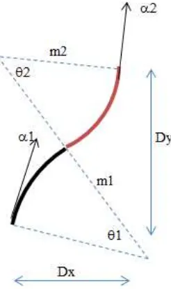
The lane centre is composed of two bend action in opposite direction as depicted in Fig. 4.

In the lane changing action, the initial angle α1 must be determined based on the final result of

prior lane border action. The direction angle α1 is

the formal direction of the entering region of the new lane. Distance Dy and Dx are calculated according to target position in the centre lane from the last position in the border.

Figure 4. Two opposite bends (m1x m2 <0) as part of lane centring level 2 robotic layer

Three geometric equations governs the lane centring in Fig. 4 are

(5)

The set of equations (5) that governing the lane centre has four unknown parameters, i.e. two rotation radius m1 and m2 and two rotation angle

θ1 and θ2. Taking one of these parameters as an

input then the formulation of lane centring is completed. This input parameter should be determined by the more intelligent sub layer in the lane changing action.

V. CONCLUDING REMARKS

The continuous two dimensional topography model was discussed in this article. This relatively new model has advantageous than the common grid structure based topography model in more detail modelling of different size traffic participant and the more realistic movement especially in the lane change model. However, the continuous topography means also extra work in the design phase of the simulator. This paper has shown that dx/dt = {v0+ a t} sin(φ)

dy/dt = {v0+ a t} cos(φ)

φ = φ 0+ v/m Δt

x = x0+ v Δt sin{1/2 (φ+ φ0)}

y = y0+ v Δt sin{1/2 (φ+ φ0)}

α1 + α2 = θ1 + θ2

[sin θ1 sin α1 + ( 1 –cos θ1) cos α1 ] m1 + [sin θ2 sin α2 + ( 1 –cos θ2) cos α2 ] m2 = Dx

the simple action of lane changing becomes a complex action in the new topography model. Fortunately, splitting-up complex actions into small and easier action that will be used in other complex action is possible and yields a very promising work. This work is following the footprint of Ulf Lotzmann’s ambitious work which started about half decade ago in Germany. For further research all actions in the behaviour layers of the agent model will be completed.

ACKNOWLEDGMENT

Thanks to LP2M UAI for funding this paper via International Seminar Grant. Thanks to Ulf Lotzmann for inspiring the ingenious idea of continuous topography and for using some figures.

REFERENCES

[1] H. T. Fritzsche, “A model for traffic simulation”, Traffic Engineering & Control 35(5), pp. 317-321, May 1994

[2] M. Brackstone, M. McDonald “Car-following: a historical review”, Tranportation Research Part F 2, Elsevier Science Ltd., p. 181-196. 1999

[3] J. J. Olstam, A. Tapani “Comparison of car -following models”, VTI medelande 960A, Swedish National Road and Transport Institute, 2004 [4] K. Nagel, M. Schreckenberg, “A cellular

automaton model for freeway traffic”. In Journal de Physique I, France, 2, pp. 2221-2229, 1992

[5] M. Rickerta, K. Nagel, M. Schreckenberg, A. Latour, “Two lane traffic simulations using cellular automata” LANL Report No. LA-UR 95-4367, 1995

[6] J. Esser, M. Schreckenberg, “Microscopic simulation of urban traffic based on cellular automata”, in International Journal of Modern Physics C, Vol. 8 No. 5, pp. 1025-1036 , 1997 [7] B. Burmeister, A. Haddadi, G. Matylis,

“Application of multi-agent systems in Traffic and transportation” in Software Engineering, IEE Proceedings, Vol. 144 (1), pp.51-60, 1997

[8] F. Klugl, H. Wahle, A. L. C. Bazzan, M. Schreckenberg, “Towards anticipatory traffic forecast- modelling of route choice behaviour”, in Proceeding of Workshop ‘Agents in Traffic Modelling’ , 2000

[9] A. L. C. Bazzan, F. Klugl, Multi Agent Systems for Traffic and Transportation Engineering, Information Science Reference, 2009

[10] J. Dijkstra, A. J. Jessurun, H. J. P. Timmermans, “A multi-agent cellular automata mode of pedestrian movement”, in Pedestrian and Evacuation Dynamics (Eds: M. Schrekenberg and S. D. Sharman), Springer-Verlag, 2001

[11] U. Lotzman, “ Design and Implementation of a framework for the integrated simulation of traffic participants of all types”, In Proceeding of the 2nd European Modelling and Simulation Symposium, 2006