Political Pressures and the Choice of the
Optimal Monetary Policy Instrument
James P. Cover and David D. VanHoose
This paper extends Cukierman’s (1992) model of monetary policy discretion, private information, and credibility to an environment in which the quantity of money is endogenous and in which a monetary authority must choose between bank reserves or an interest rate as its instrument of monetary policy. This model is used to explore the determinants of credibility for the alternative policy instruments and to evaluate the manner in which political pressures on a monetary authority can influence the authority’s instrument choice. A key implication of the model is that such political pressures can influence the credibility of monetary policy differentially depending upon the choice of policy instrument, thereby inducing a monetary authority to choose an instrument that otherwise would fail to meet standard Poole (1970) criteria. © 2000 Elsevier Science Inc.
Keywords: Optimal monetary policy; Monetary policy instruments; Monetary politics
JEL classification: E52; E58
I. Introduction
Why do nearly all central banks use an interest rate as the monetary policy instrument? According to the instruments-targets literature, a central bank’s optimal instrument of monetary policy depends on the magnitudes of macroeconomic parameters and the relative sizes of the variances of structural disturbances. Specifically, since Poole’s (1970) original analysis, this literature [e.g., Friedman (1975), McCallum and Hoehn (1983), and Benavie and Froyen (1983)] uniformly concludes that an interest-rate instrument is preferred to a bank-reserve (or monetary-aggregate) instrument if the variance of real expenditure disturbances is sufficiently small relative to the variance of financial-sector disturbances. Nevertheless, central banks in Europe and Asia consistently have used
College of Commerce and Business Administration, University of Alabama, Tuscaloosa, AL.
Address correspondence to: Professor David D. VanHoose, College of Commerce and Business Adminis-tration, University of Alabama, Box 870224, Tuscaloosa, AL 35487-0224, USA.
interest-rate instruments— even during periods in which Poole’s original condition prob-ably has not been satisfied. In addition, even though Fair (1984) finds that simulations of Poole’s criteria for the late 1970s generally support the use of an interest-rate instrument by the Federal Reserve, in 1979 the Fed switched to a reserve instrument.
Carlstrom and Fuerst (1995) propose a very different explanation that might help to explain the widespread use of an interest rate instrument even under circumstances in which the standard Poole rule is violated. They consider a model in which cash-in-advance constraints and portfolio rigidities produce distortions that can make a competitive equilibrium Pareto inefficient. Pegging the nominal interest rate eliminates these distor-tions and, therefore, is the optimal monetary policy. The reason is that an interest rate peg permits greater output responses to real shocks, thereby allowing agents greater flexibility to maximize their lifetime utility levels.
This paper extends the literature about the widespread central bank use of an interest-rate instrument by presenting a model that shows that the variability of political pres-sures— or, more generally, the variability of any factors that influence central bank preferences— can influence instrument choice. In contrast to Carlstrom and Fuerst, the rationale we suggest for why central banks typically use an interest-rate instrument mirrors the traditional Poole approach in which a central bank seeks to stabilize inflation and real output in light of nominal shocks that have short-term real consequences. Nevertheless, the explanation we propose yields the standard Poole criterion only as a special case that emerges in the absence of variable political pressures. We are able to explain why an interest-rate instrument typically is more widely used when there are variable political pressures, and we can provide a rationale for why a central bank temporarily might switch to a reserve instrument, as the Fed did from 1979 until roughly 1982. Our explanation for these phenomena stems from developments in the recent literature on monetary rules, discretion, and credibility [e.g., Kydland and Prescott (1977), Barro and Gordon (1983a, 1983b), Persson and Tabellini (1990), and Cukierman (1992)]. It also draws on the political-monetary-economy literature as exemplified by the contri-butions of Havrilesky (1987, 1993), who identifies structural elements, political linkages, and even personal characteristics that appear to have motivated Federal Reserve decision-making.
The paper extends Cukierman’s (1992, Chap. 9) basic model of private information on changing objectives, discretion, and credibility. Following Friedman (1975), we consider a setting in which the monetary authority does not directly control a monetary aggregate. Hence, the model central bank, like those in the real world, must choose between either an interest-rate or a bank-reserve instrument of monetary policy. We demonstrate that whenever monetary policy is subject to control errors that real-world central banks also experience, the variability of political pressures can play a crucial role in influencing the choice of a monetary-policy instrument. Within the present model, as in Poole’s, the shapes and relative variations in the positions of the IS and LM schedules influence a monetary authority’s choice and day-to-day maintenance of a policy instrument. Never-theless, the variability of political pressures can, because of its effects on central bank credibility, easily tilt the monetary authority toward the use of an interest-rate instrument instead of a reserve instrument.
that pushes a conservative central bank toward using an interest-rate instrument is the variability of political pressures combined with lower instrument control errors relative to the control errors associated with a reserve instrument. If the variance of political pressures is sufficiently high, whereas the variance of control errors under an interest-rate instrument is sufficiently low relative to that under a reserve instrument, then a conser-vative central bank may prefer an interest-rate instrument.
Stated differently, if the variance of control errors with a reserve instrument is sufficiently large, then the central bank loses credibility in the face of variable political pressures. Such political pressures complicate private agent learning and thereby can make a reserve instrument less desirable than an interest-rate instrument even if the latter is preferred according to standard Poole criteria. Hence, this paper’s analysis implies that a relatively conservative central bank, such as the Federal Reserve, normally uses an interest-rate instrument in part because it gains credibility from using the instrument that can be implemented with greater precision. However, if there are no variable political pressures, the increased precision obtained by using an interest rate instrument is much less important.
II. The Model
Cukierman (1992) generally considers an infinite-horizon policy problem. For purposes of this paper, we can make all our basic points in a two-period setting [see Cukierman (1995) for a similar two-period approach]. The structural macroeconomic model consists of the following equations:
yt5a~pt2pt e!
; t51, 2; a .0; (1)
yt52b~rt2pte!1ht; b .0; (2)
mt2pt5yt2frt1nt; 0,f ,1; (3)
mt5jht1krt;j .0; 0,k ,1; (4)
ht5hˆt1zt; (5)
where
yt [ deviation of output growth from its steady-state value at time t,
rt [ deviation of the nominal interest rate from its steady-state value at time t,
mt [ deviation of nominal money growth from its steady-state value at time t, pt [ deviation of the inflation rate from its steady-state value at time t,
ht [ deviation of the growth rate of bank reserves from its steady-state value at time
t, andht,nt, andztare white-noise disturbances.
The superscript “e” denotes the expectation of a variable, conditioned on available information, and hˆtis the central bank’s planned path for reserve growth. All disturbances
are independently distributed, serially uncorrelated shocks with zero means and finite variances. The two periods of the model are 1 and 2.
income-expenditure equilibrium (IS) condition, in which desired spending on real output depends negatively on the real interest rate. Equation 3 expresses the public’s desired growth of real money balances, while Equation 4 expresses the determinants of the growth rate of the nominal money stock. Equation 5 defines the growth rate of bank reserves to be the sum of the central bank’s planned growth and random disturbance,zt, which reflects the
central bank’s less-than-perfect control over total reserves. Below it is assumed that the variance of the control error might depend upon the monetary authority’s chosen instru-ment [see Board of Governors of the Federal Reserve System (1981) for discussion of the different sources of reserve volatility under alternative instrument choices]. Hencezt
r
is the control error under the interest-rate instrument, whereaszt
h
is the control error under a reserve instrument. The variances of these disturbances are denotedszr
2
andszh 2
, respec-tively.
In the spirit of Cukierman (1992), the central bank’s intertemporal objective reflects a desire to expand output growth beyond a target level while simultaneously maintaining minimal inflation (inflation smoothing). As pointed out by Balke and Emery (1994) and Svensson (1999), the assumption that the central bank engages in inflation smoothing (rather than price level smoothing) can make a significant difference in the conclusions forthcoming from an optimal-policy analysis. This paper assumes an inflation-smoothing objective because statements by central banking officials imply that inflation smoothing is a key objective.
The central bank’s objective is to minimize
L15E1$x1~y*2y1!1~1/ 2!p211G@x2~y*2y2!1~1/ 2!p22#%; (6)
whereGis the discount factor and
xt5A1gt; A.0 (7)
and where
g15m1, and (8a)
g25rm11 «2. (8b)
Generally,m1and«2are any random factors, which could well include shifts in beliefs
of or in the composition of the board governing the central bank’s policymaking appa-ratus. In light of Havrilesky’s (1987, 1993) work, this paper envisions these disturbances as arising primarily from pressures placed on the central bank by politicians. Thus, we shall refer to them as “political-pressure” shocks, even though a portion of these distur-bances can originate from other, nonpolitical sources. Because these disturdistur-bances can come from government efforts to persuade or coerce central bank officials during informal contacts—such as phone calls, private meetings, and the like—it is assumed that they occur after the beginning of each of the two periods and remain the central bank’s private information throughout the time horizon of the model.
Following Cukierman, the loss function in Equation 6 assumes that the policymaker wishes to prevent output from falling below y*. Thus, in contrast to the analysis of Barro and Gordon (1983), the variance of output does not influence the policy loss.
desires to place on output expansions. Political pressures arise, however, via the innova-tions m1and «2that capture the extent to which the monetary authority “caves in” to
coercive threats from political sources. To capture the likely persistence of the effects of such coercion, the m1political disturbance that occurs in Period 1 persists partially into Period 2.
Note that in principle it would be possible to follow the work of Fratianni et al. (1997) [which stems in part from the work of Walsh (1995)] by modeling the process through which m1 and «2are determined. This would require developing a more sophisticated
description of the interaction between the government and the monetary authority. The goal of this paper, however, is to analyze the fundamental implications of political pressure variability for the optimal instrument choice, rather than to model its source. Consequently, it is assumed thatm1and«2are white-noise, finite-variance disturbances.
III. The Case of an Interest-Rate Instrument
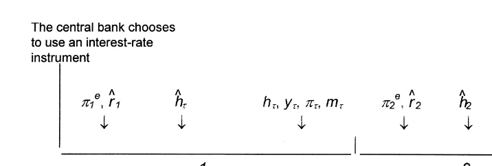
If the Fed uses the interest rate as its policy instrument, then it adjusts reserve growth each period in an effort to produce interest rates that are consistent with its objective. Figure 1 presents the timing of the model for this instrument choice. Just as the period begins the central bank chooses to use the interest-rate as its policy instrument. Then, shortly after the beginning of a period, the central bank experiences a political shock. Subsequently, private agents form their inflation expectation, and the central bank determines the optimal planned interest rate, rˆt, in light of this expectation. As a discretionary policymaker, the
central bank takes private-sector expectations of inflation as given when determining the optimal interest rate. After the central bank determines the intended value of the interest rate, the IS shock (ht) and LM shock (nt) occur. The central bank then conducts
open-market operations to adjust reserve growth in an effort to achieve the planned interest-rate setting; that is, it determines the value of hˆt. Its ability to achieve its intended
reserve growth path is imperfect, however, so a disturbance to reserves (zt r
Finally, after any interest-rate deviations occur and all decisions have been made, output growth, inflation, and money growth are determined. Then the central bank’s loss is realized. Note that we do not provide an optimizing framework for the central bank’s two-period planning horizon, nor do we permit the central bank to switch instruments after the first period. Although we believe that both issues would be interesting extensions of our model (see Section VI), our more limited goal is to understand the role that the variability of political pressures plays in a more constrained framework.
Neither the political-pressure disturbances nor the central bank’s policy error are observable to private agents. In the first period, private agents expect that these shocks will equal zero. In the second period, however, private agents use the information content in the first-period deviation of the interest rate from the value that they had anticipated to infer the most likely magnitude of the first-period political-pressure shock. They then use this inference to forecast the second-period political-pressure shock. Consequently, the central bank’s optimal policy choice during the first period influences private agents’ second-period inflation expectation. It is this aspect of the model that makes the central bank’s policy choices for the two periods interdependent.
As shown in an appendix that is available upon request, solving the model for the case of an interest-rate instrument yields the following solutions for the interest rate, output growth and the inflation rate in Periods 1 and 2:
r1r5a~12b21a2rcu
is the regression coefficient for the signal-extraction problem that private agents must solve to form the optimal inference of m1given their observation of r12
E(r1uI1).
controllability errors. If the policy instrument is the interest rate in the Poole model, then once the central bank chooses its interest rate target, it cannot achieve the desired target unless it can intervene in financial markets after the IS and LM shocks are realized. Thus, in the Poole framework neither IS nor LM shocks can affect the equilibrium rate of interest under an interest-rate instrument, which is why only IS shocks influence equilibrium output in Poole’s model.
The present model is more realistic than Poole’s in two respects. First, here it is assumed that the central bank cannot directly control the money stock, so that it must choose between an interest-rate or reserve instrument. Second, here it is assumed that the central bank does not have perfect control over either policy instrument. Nevertheless, when the central bank uses the interest rate as its policy instrument, it still chooses the target value of the rate of interest before the IS and LM shocks are realized. As in Poole’s simpler IS-LM analysis, the central bank cannot implement its policy until after the IS and
LM shocks are realized. Once these shocks are realized, it attempts to inject sufficient
reserves into financial markets to achieve the desired interest rate. Because it does not precisely know the required magnitude of the reserve injection, the realized rate of interest differs from the target value of the rate of interest. Consequently, the disturbances that affect the controllability of reserves (z1r andz2r) appear in Equations 9 and 12, but the IS
and LM disturbances do not.1
Hence, the approach of this paper captures key aspects of actual Federal Reserve behavior when it uses an interest-rate instrument. The Federal Open Market Committee sets the target value of the federal funds rate. Each day, the Trading Desk at the Federal Reserve Bank of New York buys or sells U.S. government securities in quantities that its believes will keep the federal funds rate close to its target value. If one examines historical daily data on the federal funds rate, however, one sees that the rate rarely exactly equals its target value.2
The parameterc, which may be rewritten as {11(uz2/um2)(szr2/sm2)}
21, depends upon
the public’s perception of what has caused the rate of interest to differ from its expected value based upon its knowledge of the variances of the political pressure and instrument control error disturbances,sm
2
andszr 2
. That is, neithercnorumdepends upon the current
relative weights that the central bank places on output and inflation in its loss function (6). Instead, these parameters depend on the ratio of the variances,sm2andszr2, as well as terms
that represent the slopes of the IS, LM, and aggregate supply schedules. As (szr
2
/sm 2
) approaches infinity,cand (c/um) both approach zero. In this case, private
agents behave as if there are no political pressure disturbances (because they act as though sm250). Therefore, they attribute all unexpected changes in the rate of interest to control
errors. Notice from Equations 12 and 13 that ifc5(c/um)50, then instrument control disturbances,z1
r
, would not affect the interest rate and output during period 2, whereas a political pressure disturbances, m1, would have its full effect. Similarly, notice from
1Because our approach follows Friedman (1975) and examines the instrument choice problem in a
framework in which the quantity of money is endogenous, the model could be extended to a consideration of issues related to intermediate monetary targeting. However, such issues are outside the scope of this paper.
2Indeed, there is a literature on daily variability of the federal funds rate; notable contributions are Cook and
Equations 10 and 11 that ifc5(c/um)50, then political pressure disturbances (if they
were to occur) would have their full effect on output and inflation during Period 1. As (szr
2
/sm 2
) approaches zero,capproaches unity and (c/um) approaches (b
21
a2r2G)21. As a result, 12 b21a2r2cum
21G 5
0. Notice from Equation 13 that ifc 51, then the political pressure disturbance, m1, has no effect on output during Period 2. Similarly,
notice from Equations 10 and 11 that if 12b21a2r2cum
21G 5
0, then political pressure disturbances have no effect on output and inflation during Period 1.
Because private agents use their observation of r1 2 E(r1uI1) to form the optimal
inference ofm1, the predicted value ofm1will be such that it minimizes the variance of
any forecast of the central bank’s optimal planned interest rate, rˆ1. In other words, the
values ofcandumare such that they minimize E[rˆ12E(rˆ1uI2)] 2
.
Policy is credible when economic actors believe that the monetary authority is doing what it says it is going to do. This implies that the difference between an announced target and its realized value is a natural basis for any measure of credibility. Hence Cukierman (1992) proposes using the negative of the variance of a policy forecast error as a measure of credibility. In the present case this is given by C2
r 5 2
E[rˆ12 E(rˆ1uI2)] 2
, which is the negative of the forecast-error variance experienced by private agents, conditioned on the observation of the actual Period 1 interest rate that is available at the outset of Period 2. The value of this credibility measure is given by
C2r52@um2~12c!2sm21c2uz2srz2!]. (16)
Private agents choosec andumto minimize the forecast-error variance. Thus,c is a
maximizer of C2 r
, soC2 r
/c50. This implies that Fed credibility unambiguously declines asszr2 and sm2 increase. That is, central-bank credibility would tend to fall with greater
volatility in either the central bank’s instrument control error or the political-pressure disturbance. A larger value ofareduces the central bank’s credibility, whereas a larger value ofbraises its credibility. Asarises in value, so does the temptation to try to take advantage of improved terms of the output-inflation tradeoff. For larger values of b, private spending is more interest-sensitive, so that the IS schedule is more shallow and aggregate demand is more sensitive to the effects of variations in the interest rate. This magnifies the inflationary effects of interest-rate variations, thereby making policy more credible. Similarly, as (f1 k) increases, the LM curve becomes more shallow, which reduces the amount that the interest rate changes in response to a policy control error, thereby increasing central bank credibility.
Below we will see that the above measure of credibility and how it changes is a concern of a central bank when it is deciding whether to use an interest-rate or a reserve instrument in light of its loss function in Equation 6.
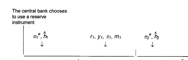
IV. The Case of a Reserve Instrument
growth. Finally, output growth, inflation, and money growth are determined. Again, the information set I1includes knowledge only of the distributions of the disturbances. For a
reserves instrument, the information set I2also includes the observation of the departure
of the reserve growth path from the value that private agents had anticipated during the first period, or h12 E(h1uI1).
Note that by using reserve growth as its policy instrument, the central bank loses a degree of freedom in its ability to adjust to shocks. Once it determines the optimal setting for reserve growth, IS and LM disturbances can, along with any policy errors, impinge on actual reserve growth. In contrast, when the central bank uses the interest rate as its policy instrument, it is able to try to adjust reserve growth as needed to achieve the optimally planned value for its interest-rate instrument. By varying reserve growth endogenously in an effort to achieve its interest-rate objective, with an interest-rate instrument the central bank automatically can respond to IS and LM shocks that otherwise would influence the market interest rate within a period. Constraining itself to a fixed, ex ante optimal reserve target path at the beginning of each period eliminates the central bank’s ability to respond to such shocks under a reserve instrument.
As outlined in the appendix, solving the model for the case of a reserve instrument yields the following reduced-form solutions for reserve growth, output growth and inflation for Periods 1 and 2:
h1h5aj21~12f 2 k!$12~bj!21@b 1 a~b 1 f 1 k!#arld21G%A
1a~bj!21@b 1 a~b 1 f 1 k!#
z$12~bj!21@b 1 a~b 1 f 1 k!#ar2ld21G%m11z1
h, (99)
y1h5a2$12~bj!21@b 1 a~b 1 f 1 k!#ar2ld21G%m 1
1@b 1 a~b 1 f 1 k!#21@bjz 1
h1~f 1 k!h
12bn1#, (109)
p1h5a$12~bj!21@b 1 a~b 1 f 1 k!#arld21G%A
1a$12~bj!21@b 1 a~b 1 f 1 k!#ar2ld21G%m 1
1@b 1 a~b 1 f 1 k!#21@bjz 1
h1~f 1 k!h
12bn1#, (119)
h2h5aj21~12f 2 k!A1ar~bj!21@b 1 a~b 1 f 1 k!#$~12l!m
12ld21z1 h%
1a~bj!21@b 1 a~b 1 f 1 k!#«
2, (129)
y2h5a2«21a2r~12l!m12a2rld21zh11@b 1 a~b 1 f 1 k!#21 product ld21is the regression coefficient for the signal-extraction problem that private agents must solve to form the optimal inference of m1given their observation of h12
E(h1uI1). For reasons similar to those stated above, the values ofl andd do not depend
upon the relative weights on output and inflation in the loss function (Equation 6), rather only onsm
2
,szh 2
, and terms that represent the slopes of the IS, LM, and aggregate supply schedules. As in our analysis of an interest rate instrument, the timing assumptions and forth-coming solutions are similar to those in Poole’s original framework. Poole’s analysis assumes that the money stock could be used as a policy instrument and that the central bank chooses the target value of the money stock before realization of the IS and LM shocks. Thus, both shocks affect the equilibrium values of the interest rate and output. In our more general framework in which growth of bank reserves instead of the money stock is the policy instrument, the central bank also chooses its reserve instrument before the IS and LM shocks are realized. Once bank reserves are set, both the IS and the LM shocks affect the equilibrium level of output, as in Poole’s model.
In comparing Equations 99through 159with Equations 9 through 15, note thatl5c whenever the variance of the monetary control disturbance does not depend upon the operating instrument.3That is,l5cif and only ifszh
2 5 szr
2
. This implies (as is discussed further in Section 5, below) that the choice of policy instrument will depend only on the relative sizes of the IS and LM curve disturbances if the monetary control disturbance is the same under both operating instruments.
This can be seen by assuming thatm15«25z1 pressures and instrument-control precision are irrelevant. In this situation, the remainders of Equations 10, 11, 13, and 14 show that output and inflation depend only on the IS disturbance under an interest-rate instrument, whereas the remainders of Equations 109, 119, 139, and 149indicate that both the IS and the LM disturbances affect output and inflation under the reserve instrument. Hence, the instrument-choice problem reverts to a problem similar to that examined by Poole if the political and monetary control disturbances are eliminated. This special case, therefore, replicates Poole’s analysis, at least within our two-period framework. In general, because private agents chooselanddto yield the best prediction ofm1, the
values of these parameters minimize the policy-prediction-error variance, and therefore, maximize the credibility measure, which is given by
C2
21G]. Likewise the expression forlcan be
rewritten asl5(duz)2s
2]. These rewritten expressions make it obvious thatl5candu
m5
SinceC2 h
/l50, credibility again declines unambigously with greater volatility in either the political-pressure disturbances or the central-bank instrument control error. In addi-tion, the central bank’s credibility is a declining function ofd.
As in the interest-rate-instrument case, a rise inaincreases the temptation to inflate, thereby reducing the central bank’s credibility. Also, a rise inbflattens out the IS schedule and increases the inflationary effect of a shift in the LM schedule caused by an increase in reserve growth, which raises credibility. Because reserve growth has greater direct effects on the LM and aggregate demand schedules if the value ofjis higher, an increase in this parameter also leads to improved credibility. Higher values of f and k imply reductions in the interest-sensitivity of money demand and supply, respectively, which make the LM schedule more shallow and reduces the inflation impact of an increase in reserve growth, thereby reducing the central bank’s credibility.
Finally, credibility under a reserve instrument (Equation 169) is measured in different units than credibility under an interest-rate instrument (Equation 16). But if we multiply Equation 169by the factor uz
2
, we express the reserve-instrument credibility measure in units that are the same as the credibility measure for the interest-rate instrument. These two credibility measures yield identical values ifszh
2 5 szr
2
. Thus, the instrument with the lower control error variance yields greater central-bank credibility. When there are variable political pressures, this fact can have a relatively large influence on the instrument of monetary policy chosen by the central bank.
V. The Optimal Choice of a Monetary Policy Instrument
Now that we have considered a central bank’s optimal setting of both and interest-rate instrument or a reserve instrument given its private information about political pressures, we can now to determine how a central bank chooses its instrument. In this model, the existence of variable political pressures influences the central bank’s choice of a policy instrument. The source of this influence is through the information received by private agents. If there is an unanticipated change in a policy instrument, private agents are able to make inferences about the changing objectives of the central bank. Such inferences influence their expectations of inflation during both periods, thereby altering the realizations of inflation and output in each period. This section shows that this difference in the realizations of output and inflation under the two policy instruments implies that variable political pressures causes a modification of the standard Poole criterion for the optimal instrument choice.
Replicating the Poole Rule
The central bank chooses its instrument before it observes political-pressure disturbances. Consequently, we evaluate the central bank’s expected losses over the model’s two-period horizon at the end of period 0 before the realization of the political shock in Period 1. It is useful to express the loss as:
L05E0$x1~y*2y1!1~1/ 2!p211G@x2~y*2y2!1~1/ 2!p22#%;
51~1/ 2!@E0~p12p1
e!21GE
0~p22p2 e!2#
1~1/ 2!$@E0~p1e!#21G@E0~p2e!#2%
Equation 69 presents the expected loss as the sum of three components. The first is the discounted sum of conditional inflation variances over the two periods. The second is the discounted sum of the squared mean inflation biases. The third is the discounted sum of expected output losses over the model’s two-period horizon.
It is possible to evaluate the factors that influence the central bank’s instrument choice in the presence of private information about political pressures by comparing the values that these components assume for each instrument, which may be computed using the model solutions derived in Section III. But because doing so is very complicated, it is more appropriate to consider each of these three components separately. Below it is demonstrated that if political pressures are not variable, then differences between the second and third components, the mean inflation biases and output losses, disappear when comparing losses for the two instruments. This leaves only differences in expected losses due to the variance of inflation and thereby replicates the Poole rule for the optimal instrument choice. Hence our discussion will begin with losses from inflation variability.
Inflation Variability. A key implication that our model shares with other models of
optimal monetary policy is that a central bank faces a tradeoff among its output and inflation objectives when it makes its policy instrument choice. In our model, this is determined by the magnitude of the parameter A, which measures the central bank’s true underlying preference about output expansions relative to inflation. A central bank that exhibits a relatively small value for A at the end of period 0 has maintained a considerable degree of “conservatism” to that point, possibly because it has not been subjected to political pressures favoring monetary policy “ease” in previous periods. In contrast, a “liberal” central bank whose objectives at the end of period 0 show a strong bias toward output growth would exhibit a relatively large value for A.
Here we focus on a conservative central bank, which places considerable weight on the inflation component of its loss function and thereby seeks to choose the policy instrument that produces smaller mean inflation and lower inflation uncertainty. To evaluate the instrument-choice implications for inflation uncertainty, define the discounted sum of inflation variances over the two periods (the first component of the total loss in (Equation 69) to be V5V11 GV2[E0(p12p1
e
)21 GE0(p22p2 e
)2. For the case of an interest-rate instrument, this inflation variability component of the total policy loss is given by
Vr5~11G!$@b 1 a~b 1 f 1 k!#22b2j2s
In the case of a reserve instrument, the inflation variability portion of the loss is equal to
Vh5~11G!@b 1 a~b 1 f 1 k!#22@b2j2s
This implies that the condition for Vr, Vhis given by
If there are no political-pressure shocks, so thatsm 2 5
0, then this condition reduces to
sh2,a2b2$sn21j2~szh2 2s2zr!%/~11a!b@~11a!b 12a~f 1 k!#, (19)
which is the basic “Poole rule” for this model.
The second term inside the braces on the right-hand side of Equation 19 represents the effect of control precision on the optimal instrument of monetary policy. If the variance of the monetary-control disturbance is larger under a reserve instrument than under an interest-rate instrument, then the right-hand side of Equation 19 increases, making it more likely that the Poole rule will imply that the interest-rate is the optimal instrument for monetary policy. As the money-stock multiplier, j, increases, the importance of any difference in the variance of the control errors increases.
But if the control disturbances under the two instruments have the same variance,szh2
5szr 2
, then the variance of the IS disturbance must be lower than the variance of the LM disturbance for the interest-rate instrument to be preferred (becausea2b2/(11a)b[(11 a)b12a(f1k)],1).
The other properties of Equation 19 are standard. As the IS schedule becomes more shallow (bincreases), as the LM schedule steepens (f1kdecreases) and as the aggregate supply schedule becomes more shallow (aincreases), the right-hand side of Equation 19 becomes larger, making it more likely that the interest-rate instrument is preferred.
For the purposes of argument, assume that the Poole criterion causes the central bank to be indifferent between the two instruments. Forsm2.0, it then follows from Equation
18 that inflation uncertainty is lower under an interest-rate instrument (Vr,Vh) if 12 (bj)21[b 1a(b 1f1 k)]3 ar2ld21G ,12b21a2r2cum
21G
. But this condition is equivalent touzcum
21.ld21, which holds only ifs zr 2 , s
zh
2. Given the variance of the
political-pressure disturbance, the instrument with the lower control-error variance thereby yields lower inflation variability. This is true because the instrument with greater control precision improves central bank credibility. Hence if the interest-rate instrument has the lower control-error variance, then the existence of political-pressure disturbances makes its more likely that the interest rate will be the optimal instrument of monetary policy for a conservative central bank.
Mean Inflation. With either instrument, from the perspective of the very beginning of
Period 1 (just before the political shockm1 is realized), anticipated mean inflation for
Period 2 is equal toaA. Consequently, the mean-inflation loss comparison hinges simply
on a direct comparison of p1re 5 a
(1 2 b21a2rcu m
21G
)A and p1he 5 a$1 2 ~bj!21
@b 1 a~b 1 f 1 k!#arld21G%A.
First note that if there is no variability of political pressures, thensm250, which causes cum
215ld215
0, andp1re5p 1 he5a
A. The monetary authority is indifferent between
the two instruments as far as the mean inflation loss is concerned. Otherwise, the comparison implies thatp1re,p1heforszr2 ,szh2. The instrument with the lower control
Output Losses. A conservative central bank places relatively little weight on output
losses in either period. Nevertheless, to evaluate the output-loss factors that influence a conservative central bank’s choice between the alternative monetary policy instruments, it is helpful to write the output-loss component of Equation 69 as Ly 5 L1
y 1 G
individually. It is straightforward to show that the second-period output loss component with an interest rate instrument is L2
yr 5 analogous expression with a reserve instrument is L2
yh5 Consequently, if the variance of the political disturbance is zero, then instrument choice does not affect second-period output losses. Otherwise, L2
yr,
. Second-period output losses are lower for the instrument with the larger control error.
The first-period output losses are L1 yr5 does not affect this output loss if the variance of political disturbances is zero. Otherwise we have L1 with the larger control error variance yields the lower first-period output loss.
Some Implications
Regime Switching. The previous section shows that if the political pressures on a
central bank are not variable (sm 2 5
0), then the Poole rule for the present model is Equation 19 above. If the variance of the IS disturbance (sh
2
) is sufficiently small, then the rate of interest is the preferred instrument of monetary policy. If there are variable political pressures, however, then the greater precision with which policy can be implemented under an interest-rate instrument (szh
2 . szr
2
) generates a reduction in inflation losses. The trade-off is higher output losses under an interest-rate instrument.
Hence, a conservative central bank is more likely to choose an interest rate instrument as the variability of political pressures increases. Suppose, however, that there is an increase in concern over inflation that reduces the variability of political pressures, as may have been the case in the US during the late 1970s. In this situation, the interest-rate instrument loses some of its credibility relative to the reserve instrument, making it more likely that a conservative central bank will choose a reserve instrument.
Correlation Between Mean Inflation and Inflation Uncertainty. If the Poole rule for
the present model (Equation 19 above) produces central bank indifference between the two instruments, then the instrument that produces lower expected inflation also produces the lower conditional variance of inflation. Thus, mean inflation and inflation uncertainty are positively correlated.
Finally, Cukierman offers an explanation based on the existence of asymmetric informa-tion: A reduction in the variance of monetary control errors reduces the central bank’s gains from inflating and thereby leads to lower monetary growth at the same time that it reduces inflation uncertainty.
The explanation for the positive relationship between inflation and inflation uncertainty offered in this paper differs from each of the above explanations, although it is similar to Cukierman’s explanation in that it relies on the existence of asymmetric information. But here the positive relationship between inflation and inflation uncertainty occurs because of the interplay between variable political pressures and differences in instrument precision. If there are no variable political pressures, both mean inflation and inflation uncertainty are independent of the central bank’s policy instrument, and the present explanation of a positive relationship between the two disappears.
VI. Conclusion
The instrument choice model developed in this paper has two key implications. First, the standard Poole criterion for a central bank’s choice of the optimal monetary policy instrument represents only one aspect of a central bank’s policy problem when it faces political pressures. When the full effects of such external pressures are the central bank’s private information, a central bank also must take into account the credibility implications of its instrument choice. Second, to the extent that political-pressure and credibility considerations predominate in determining a central bank’s instrument choice, the model indicates that a conservative central bank may value the credibility-enhancing precision of a monetary policy instrument as well as its macroeconomic stabilization properties. To the extent that using an interest-rate instrument yields greater policy precision as compared with the implementation of a reserve-oriented policy procedure, this could produce a natural bias toward adopting an interest rate as the instrument of monetary policy. If the credibility gains from using an interest-rate instrument are sufficiently large, then a central bank would continue to use this instrument even if it might be able to achieve a stabilization gain by adopting a reserve-based approach to conducting monetary policy.
This leads to the second issue that we are considering in further work. Our model in the present paper assumes that political-pressure shocks are incorporated directly into the central bank’s output-inflation preferences. If the central bank’s preferences are distinctive from those of the government officials who subject the central bank to such pressures and if the central bank possesses private information about its policy errors (thezdisturbances in our model), then the potential exists for independent central bank policy strategies to partially offset the effects of such governmental pressures. This points to a potentially fruitful extension of our model, in which both government officials and central bank policy makers have their own private information sets. Government officials could use structural control over certain aspects of central-bank independence and an optimal degree of pressure to impinge on the central bank’s objectives, but in the absence of complete information about the precision with which the central bank can conduct policy and about the central bank’s true objectives. The central bank, in turn, would have the freedom to react to such governmental pressures by altering policy instrument settings, or even switching policy instruments.
Finally, it would be interesting to extend this model to an infinite-horizon setting. Although we believe that our two-period model captures the essential intertemporal tradeoffs that the central bank faces, an infinite-horizon environment undoubtedly would yield more general, and richer, sets of conclusions about the central bank’s instrument-choice problem in a real-world setting with no “concluding” period. We leave these and other interesting issues for future research.
We gratefully acknowledge helpful suggestions from the editor, two anonymous referees, Berthold Herrendorf, Robert Hetzel, Mark Toma, Carl Walsh, and participants in seminars at the University of Alabama, Texas A&M University, the Federal Reserve Bank of Dallas, and the University of Georgia. Any remaining errors are solely our own.
References
Balke, N. S., and Emery, K. M. Winter 1994. The algebra of price stability. Journal of
Macroeco-nomics 16:77–97.
Ball, L. June 1992. Why does high inflation raise inflation uncertainty? Journal of Monetary
Economics 29:371–388.
Barro, R. J., and Gordon, D. B. April 1983. A positive theory of monetary policy in a natural rate model. Journal of Political Economy 91:589–610(a).
Barro, R. J., and Gordon, D. B. July 1983. Rules, discretion, and reputation in a model of monetary policy. Journal of Monetary Economics 12:101–121(b).
Benavie, A., and Froyen, R. May 1983. Combination policies to stabilize prices and output under rational expectations. Journal of Money, Credit, and Banking 15:186–198.
Bennett, P., and Hilton, S. April 1997. Falling reserve balances and the Federal funds rate. Federal Reserve Bank of New York Current Issues in Economics and Finance 3.
Board of Governors of the Federal Reserve System. February 1981. Federal Reserve Staff Study.
New Monetary Control Procedures.
Clouse, J., and Elmendorf, D. 1998. Declining required reserves and the volatility of the Federal funds rate. Board of Governors of the Federal Reserve System, Unpublished Manuscript. Cook, T., and Hahn, T. November 1989. The effect of changes in the Federal funds rate target on
market interest rates in the 1970s. Journal of Monetary Economics 24:331–351.
Cukierman, A. 1995. Towards a systematic comparison between inflation targets and monetary targets. Unpublished Manuscript, Tel-Aviv University.
Cukierman, A. 1992. Central Bank Strategy, Credibility, and Independence. Cambridge, MA: MIT Press.
Devereux, M. January 1989. A positive theory of inflation and inflation variance. Economic Inquiry 27:105–116.
Fair, R. September 1984. Optimal choice of monetary policy instruments in a macroeconometric model. Journal of Monetary Economics 22:301–315.
Fratianni, M., von Hagen, J., and Waller, C. J. April 1997. Central banking as a political principal-agent problem. Economic Inquiry 35:378–393.
Friedman, B. October 1975. Targets, instruments, and indicators of monetary policy. Journal of
Monetary Economics 1:443–473.
Havrilesky, T. M. 1993. The pressures on American monetary policy, Norwell, MA: Kluwer Academic Publishers.
Havrilesky, T. M. August 1987. A partisanship theory of fiscal and monetary regimes. Journal of
Money, Credit, and Banking 19:308–325.
Holland, A. S. January 1993. Uncertain effects of money and the link between the inflation rate and inflation uncertainty. Economic Inquiry 31:39–51.
Kydland, F. E., and Prescott, E. C. June 1977. Rules rather than discretion: The inconsistency of optimal plans. Journal of Political Economy 85.
McCallum, B., and Hoehn, J. G. February 1983. Instrument choice for money stock control with contemporaneous and lagged reserve requirements. Journal of Money, Credit, and Banking 15:96–101.
Persson, T., and Tabellini, G. 1990. Macroeconomic Policy, Credibility, and Politics. London: Harwood Publishers.
Poole, W. May 1970. Optimal choice of monetary policy instruments in a simple stochastic macroeconomic model. Quarterly Journal of Economics 84:197–216.
Rudebusch, G. April 1995. Federal funds interest rate targeting, rational expectations, and the term structure. Journal of Monetary Economics 35:245–274.
Sellon, G., Jr., and Weiner, S. 4th Quarter, 1996. Monetary policy without reserve requirements: Analytical issues. Federal Reserve Bank of Kansas City Economic Review. 81:5–24.
Svensson, L. August 1999, Part 1. Price-level targeting versus inflation targeting: A free lunch?
Journal of Money, Credit, and Banking 31:277–295.
Thornton, D. January/February 1988. The borrowed-reserves operating procedure: Theory and evidence. Federal Reserve Bank of St. Louis Review. 70:30–50.
VanHoose, D., and Humphrey, D. (in press). Sweep accounts, reserve management, and interest rate volatility. Journal of Economics and Business.