Increasing Liquidity and the Declining
Informational Content of the Paper-Bill
Spread
J. Peter Ferderer,* Stephen C. Vogt and Ravi Chahil
The paper constructs a theoretical model to show that the reduced-form relationship between the paper-bill spread and its determinants is sensitive to the substitutability between paper and bills in investors’ portfolios. Using the trend ratio of bill to paper volume outstanding as a proxy for relative liquidity of commercial paper, we provide evidence that the ability of the spread to embody important information fell as liquidity of the paper market increased during the 1980s. © 1998 Elsevier Science Inc.
Keywords: Liquidity; Business cycles
JEL classification: E32, E44
I. Introduction
Considerable attention has been devoted to analyzing the business cycle behavior of the spread between interest rates on commercial paper and Treasury bills. Early research in this area documented and attempted to explain the paper-bill spread’s predictive power for business cycle fluctuations.1The view that has emerged is that the spread rises prior to and during economic contractions because it embodies information about: 1) the stance of monetary policy; 2) the likelihood of default, and 3) cash flow needs linked to rising inventories.
More recent research has attempted to explain why the predictive power of the spread declined during the 1980s. One explanation suggests that, although the spread may reflect important information about monetary policy or default risk associated with financial
Department of Economics, Macalester College, St. Paul, Minnesota; Department of Finance, DePaul University, Chicago, Illinois; Department of Economics, Clark University, Worcester, Massachusetts.
Address correspondence to: Dr. J. P. Ferderer, Department of Economics, Macalester College, 1600 Grand Avenue, St. Paul, MN 55105.
1Relevant papers include Cook (1981), Rowe (1986), Stock and Watson (1989), Bernanke (1990), Friedman and Kuttner (1992, 1993), Kashyap et al. (1993), Bernanke and Blinder (1993).
Journal of Economics and Business 1998; 50:361–377 0148-6195 / 98 / $19.00
crises, these forces have recently played a diminished role in the business cycle [see Friedman and Kuttner (1994) and Emery (1996)]. Also, it has been argued that changes in the supply of commercial paper and Treasury bills, unrelated to business cycle conditions, have played a more dominant role in driving the spread.
An alternative explanation for the decline in the spread’s predictive power has its origins in the dramatic rise in liquidity of the paper market over the past two decades. As Stigum (1990) has observed:
A commercial paper trader’s primary responsibility is to assist issuers, but he also has a second responsibility, to provide liquidity to investors. More than any other aspect of the commercial paper market, it is the secondary market that has, in recent years, been developed. [Stigum (1990, p. 1051)]
As the liquidity of commercial paper rises, it becomes a closer substitute to Treasury bills in investors’ portfolios. As a result, shocks to either the paper or bill market cause rates in both markets to change proportionately. Thus, the spread is less sensitive to changes in market conditions linked to the business cycle.
Although this explanation has been discussed in the literature, it has not been formally analyzed.2The objective of this paper is to fill this void in the literature. We do so by constructing a theoretical model which shows precisely how the relationship between the spread and its determinants is conditional on the substitutability between paper and bills in investors’ portfolios. Our second contribution is empirical. Using two different variants of the trend ratio of bill to paper volumes outstanding as proxies for the relative liquidity of commercial paper, we show that the coefficients linking the spread to its determinants fall as the liquidity of commercial paper rises. Moreover, we show that the paper-bill spread contains a liquidity premium which became less sensitive to interest rate uncer-tainty during the 1980s.
The paper is outlined as follows. The theoretical model and a discussion of previous work are presented in Section II. Data and measurement issues are discussed in Section III. The results are presented in Section IV, and Section V concludes the paper.
II. Conceptual Issues
This section constructs a reduced-form model for the paper-bill spread derived from general specifications for supply and demand in the paper and bill markets. Our objective is to show that the spread’s sensitivity to exogenous changes in supply and demand declines as substitutability between paper and bills rises. The remainder of the section links the general model to previous work and discusses competing theories about the breakdown in the spread’s predictive ability.
The Model
Supply and demand for Treasury bills are expressed, respectively, as:
Bt
where rB,tand rP,tare the Treasury bill and commercial paper rates; XBStand XBDtare vectors of exogenous variables which have a systematic impact on the supply and demand for bills; a and b are vectors of structural parameters; a0, b0andhare scalar parameters; «t
BS and«t
BD
are zero-mean shocks to the supply and demand for bills. Supply and demand for commercial paper are given by:
Pt
where XPSt and XPDt are vectors of exogenous variables which impact the supply and demand for commercial paper; c and d are structural parameter vectors; co and doare scalar parameters;«t
PS and«t
PD
are zero-mean shocks to the supply and demand for paper.3 Although the demand curves are not explicitly linked to an optimization problem, it is easy to see how they could result from the wealth maximization of investors. For example, in a world with three assets—Treasury bills, commercial paper and money—the second terms on the right sides of equations (2) and (4) are the relative yields between bills and money (equation (2)) and paper and money (equation (4)) where money earns zero interest. Similarly, the third term on the right sides of equations (2) and (4) are relative yields between bills and paper.
The key parameter of interest ish—the cross-elasticity between bills and paper. It reflects the willingness of investors to substitute between paper and bills. Low substitut-ability is reflected by small values ofh. In this case, equilibrium is restored following a disturbance primarily by an interest rate adjustment in the market where the disturbance occurred. In contrast, large h implies high substitutability. In this case, equilibrium is restored following a shock to one market by yield adjustments in both markets. For example, an increase in the supply of paper causes the paper rate to rise so that investors are induced to hold less money and more paper. However, the initial rise in the paper rate is moderated by arbitrage across the paper and bill markets by investors who view these two assets as close substitutes.
In practice, four factors make paper and bills imperfect substitutes: 1) income earned from paper is taxable while bills are tax-free; 2) paper is subject to default; 3) bills provide services (e.g., banks can use bills to post margin, collateralize overnight repurchase agreements, and satisfy capital adequacy requirements) not provided by paper, and 4) bills have been more liquid than paper. If any of these factors changes, h should take on different values.
Solving for the reduced form equation for the paper-bill spread, we get4
rP,t2rB,t52azXBSt1bzXBDt1xzXPSt2dzXPDt1ut (5)
where: a 5az~co1do!/c .0;
b 5bz~co1do!/c .0;
x 5cz~ao1bo!/c .0;
3The shocks are assumed to be uncorrelated. This is a simplifying assumption and does not change the main results of the model. As we see in the empirical section below, variables used to measure the impact of a particular influence on the supply and demand in one market certainly embody information about other influences as well.
d 5d z ~ao1bo!/c .0;
c 5 h~ao1bo1co1do!1~ao1bo!~co1do!;
and the variance of the error term in the reduced form model for the spread is given by:
var~ut!5
S
Equations (5) and (6) are used in the rest of this section to discuss previous work in this area and competing explanations for the breakdown in the spread’s predictive power.
Previous Work
What factors should be included in the vectors of exogenous variables discussed above? Previous work has focused on three factors which influence the demand-side of the paper and bill markets in a way that can account for the paper-bill spread’s ability to predict business cycle movements.5First, an expectation of reduced economic activity leads to the belief that paper issuers are less likely to service their debt and, as a result, investors reduce the ratio of paper to bills in their portfolios. Second, investors may decrease the ratio of paper to bills in their portfolios as the level of nominal interest rates rise to take advantage of the tax-free nature of interest income earned on bills. If tight monetary policy causes nominal interest rates to rise prior to and during recessions, this could explain the strong predictive performance of the paper-bill spread. Finally, the paper-bill spread may contain a liquidity premium which is related to the business cycle.
In contrast to other factors, the liquidity premium has received little attention in the literature.6This is surprising given the large body of work in finance which shows that an asset’s liquidity has a significant effect on its expected return and, by implication, the spread between expected returns on assets of differing liquidity [see Amihud and Men-delson (1986, 1991); Shen and Starr (1992); Kamara (1994)]. For example, Kamara (1994) has shown that the spread between yields on relatively illiquid Treasury notes and liquid bills of equal maturity increases when interest rate uncertainty rises.7This logic suggests that the paper-bill spread might also contain an uncertainty-driven liquidity premium that rises prior to and during recessions.8
Two supply-side shocks linked to the business cycle may influence the paper-bill spread. First, tight monetary policy raises the paper-bill spread by forcing bank-borrowers into the paper market. The credit-crunch version of this hypothesis posits that tight policy produced disintermediation out of the banking industry when deposit rate ceilings were binding prior to the removal of Regulation Q [see Cook (1981) and Rowe (1986)].
5Friedman and Kuttner (1993) provide an excellent taxonomy of these effects.
6Friedman and Kuttner (1993) discuss the liquidity premium, but do not attempt to directly measure it. 7He [Kamara (1994)] argues that an asset’s liquidity premium is the product of the: a) expected length of time it takes to transact in the asset, and b) volatility of its price. The difference between note and bill liquidity premia is a function of the difference in the expected length of time to transact in each asset multiplied by asset-price uncertainty. As long as notes are less liquid, the note-bill yield spread is sensitive to interest-rate uncertainty.
Disintermediation raised paper rates relative to bill rates because funds from the banking sector flowed disproportionately into the bill market (because of the lower minimum denominations of bills) and the nonpecuniary services provided by bills (i.e., their use in posting margin, collateralizing overnight repurchase agreements, and satisfying capital adequacy requirements) limited arbitrage across the markets, thus preventing equalization of the rates. Moreover, disintermediation reduced the ability of banks to make loans and thus forced firms to issue more commercial paper.
The simple imperfect-substitutability version of the monetary hypothesis suggests that
all episodes of monetary tightening lead to higher costs of funds for banks, causing them
to restrict the supply of (and/or raise the interest rate on) bank loans [see Bernanke (1990); Kashyap et al. (1993)]. Some borrowers respond by issuing more commercial paper and, as long as paper and bills are imperfect substitutes in investors’ portfolios, the paper-bill spread rises.
A second supply-side shock which may affect the spread in anticipation of business cycles is a change in business inventories [see Friedman and Kuttner (1993); Calomiris et al. (1994)]. The primary motive for commercial paper issuance by nonfinancial firms is the financing of inventory accumulation. As firms issue more commercial paper in response to rising inventories at business cycle peaks, upward pressure is put on the paper-bill spread.
Explaining the Decline in Predictive Power
Several papers have documented the recent deterioration in the spread’s predictive power [for example, see Hess and Porter (1993); Friedman and Kuttner (1994)]. One explanation for the declining predictive power is that recent business cycle movements have been driven by shocks which do not have a strong influence on the paper and bill markets. For example, Friedman and Kuttner (1994) argued that the 1990 –1991 recession resulted from adverse supply and fiscal policy shocks which do not impact the paper-bill spread. Also, Emery (1996) observed that there has been a downward trend, dating back to the 1970s, in “point estimates of the impact of spread movements on economic activity” (p. 1). Emery did not explore the cause of this parameter instability other than to point out that the Lucas Critique was at work.9
A second possible explanation is that factors unrelated to the business cycle have played a larger role in driving the spread in recent years. For example, Friedman and Kuttner (1994) contended that idiosyncratic changes in paper and bill supplies— changes unrelated to business cycle conditions— caused the paper-bill spread to rise during the economic expansion of the late 1980s.10
A third possible explanation for the declining predictive power of the spread is that the forces driving the business cycle have not changed, but that the ability of the spread to respond to these forces has diminished due to an increase in paper market liquidity. Conceptually, this can be seen by examining the reduced form parameters in equation (5).
9Along similar lines, Hafer and Kutan (1992), and Thoma and Gray (1993) argued that the predictive power of the spread prior to the mid-1980s arose mainly from two outliers in the data: the period around the collapse of the Franklin National Bank in 1974 and 1980 when the Carter Credit controls were imposed. When these two periods are excluded, the predictive power of the spread falls considerably.
Note that shifts in market supply and demand affect the paper-bill spread as long as paper and bills are imperfect substitutes (i.e.,h, `). When the substitutability rises— due to increased liquidity of commercial paper—the spread becomes less sensitive to exogenous changes in supply and demand.11If this explanation is correct, we should observe that the reduced form parameters in equation (5) are systematically linked to paper market liquidity.12
Equation (6) reveals an additional way to test the liquidity explanation for the breakdown in the spread’s predictive performance. Note that the error term variance falls when the substitutability between paper and bills rises. If the error term in equation (5) displays heteroskedasticity induced by changes in the liquidity of paper, there is additional evidence that the decline in the spread’s predictive power resulted from a reduction in its ability to reflect supply and demand shocks.
III. Data Preliminaries
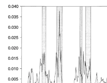
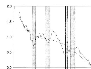
Our objective was to estimate equation (5). To do so, we followed previous work when measuring the model’s variables.13 The paper-bill spread (SPREAD) is the difference between the 6-month commercial paper and Treasury bill rates. The spread is illustrated in Figure 1 along with NBER-dated recessions (shaded regions). To gauge the stance of monetary policy, we used the spread between the 10-year Treasury bond yield and federal funds rate (SLOPE).14The spread between BAA and AAA corporate bond rates (QUAL) was used to measure default risk. To measure inventories, we used the log of real manufacturing inventories (INV). Interest rate uncertainty was quantified by fitting a GARCH (1, 1) model to daily 3-month Treasury bill yields and averaging the conditional standard deviations over the month. Because empirical relationships between liquidity premia and uncertainty are often concave, we used the log value of this series (UNCERT). To measure the relative liquidity of commercial paper, we started by taking the ratio of the quantity of bills outstanding to paper outstanding. The log of this ratio, QB/QP, is illustrated in Figure 2. As the volume of paper outstanding rises, the number of potential investors and market makers willing to take the other side of trades also rises. This reduces search costs and raises the liquidity of commercial paper.15To avoid associating tempo-rary movements in the volume ratio with changes in liquidity, we used two different measures of its trend value to measure the relative liquidity of commercial paper. The first is a polynomial time trend fit to the volume ratio, (QB/QP)
T
, shown in Figure 2. We also measured the trend by taking a moving average of the volume ratio over the previous 12 months, exclusive of the current month.
11In the limit, when paper and bills are perfect substitutes, the reduced-form parameters in equation (5) equal zero, and shifts in supply and demand have no impact on the spread. In this case, a yield increase in one market stimulates arbitrage across the markets which continues until the initial shock is absorbed by equal changes in both rates.
12Note that the second explanation requires that the substitutability between bills and paper has not declined. 13Data sources are given in Appendix 2.
14This approach is used by Blinder and Bernanke (1992), Bernanke (1990), and Kashyap, Wilcox and Stein (1993).
The trend volume ratios indicate that the liquidity of the paper market was rising up to 1989. Then, beginning in 1990, the volume ratio began to increase.16Does this indicate that paper market liquidity was falling during the 1990s? Perhaps. However, the costs associated with providing liquidity to the market are largely fixed and sunk. Thus, we should not expect that the number of dealers providing liquidity services to fall dramat-ically when the volume of paper in the market stops growing for a few years.
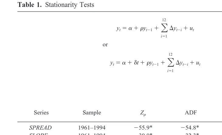
Table 1 contains stationary tests for the series. For the interest rate spread and uncertainty series, the null hypothesis is that each variable has a unit root and the alternative hypothesis is that the series is stationary around a constant mean. For inven-tories and the bill-paper volume ratio, we tested the unit root null against an alternative which specified that the series is stationary around a linear trend. The results indicate that the unit root null can be rejected at conventional significance levels for each of the spread variables and interest rate uncertainty. In contrast, the inventories series was stationary only after it had been first-differenced. Moreover, both the augmented Dickey-Fuller statistic and the exclusion test suggest that the bill-paper volume ratio is stationary around a linear trend.
16According to Friedman and Kuttner (1994), growth of the paper market slowed in the 1990s as the corporate leverage movement of the 1980s came to an end. The 1990–1991 recession also played a role. In contrast, net Treasury bill issuance expanded greatly during this period and reflected a combination of fiscal, debt-management and exchange-rate policies.
IV. Empirical Results
Preliminary ResultsOur objective was to estimate equation (5) and to examine how the coefficients evolved over time. We are particularly interested in the relationship between the coefficients and the trend volume ratios used to proxy liquidity. Due to the unavailability of data on the quantity of commercial paper outstanding prior to January 1966, we used this as the starting date for our sample. Column (1) of Table 2 presents results for the basic model, estimated with nonlinear least squares and a first-order serial correlation correction to the errors (r is the serial correlation coefficient).17Several important findings emerged.
First, the coefficient estimates generally conformed to theory and previous empirical work. The coefficient on SLOPE was positive and highly significant, suggesting that tight monetary policy is associated with a higher paper-bill spread. The weak link between the BAA-AAA quality spread is also consistent with previous work [see Bernanke (1990); Friedman and Kuttner (1993)]. The positive relationship between conditional interest rate volatility and the spread is a novel finding. It implies that the spread contains a liquidity premium which is sensitive to interest-rate uncertainty. Finally, growth of aggregate inventories was associated with a rising spread.
17As discussed below, the error terms exhibited heteroskedasticity as well as serial correlation. To obtain consistent estimates for the covariance matrix of the coefficients and robust standard errors in this case, the nonlinear least squares procedure in RATS was used along with the ROBUSTERRORS option.
It is well known that a major structural shift in U.S. money markets took place in 1979 when the Fed began to target nonborrowed reserves. To examine whether the reduced form parameters changed over the sample, we conducted a Chow test for parameter stability. Thex2statistic (CHOW) in column (1) allows us to reject the null hypothesis of parameter stability. Thus, it appears that the coefficients had significantly different values prior to January 1979 than they did after this date.
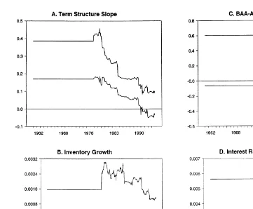
To see precisely how the coefficients evolved over the full sample, we estimated the reduced-form model using rolling regressions. The model was initially estimated over 1961:01–77:12, and then observations were added (and dropped) one at a time as we moved through the sample. Figure 3 illustrates the 95% confidence bands for each of the coefficients.
Panel A shows that the coefficient on SLOPE experienced the most dramatic and consistent change in value over the sample, falling from values between .20 and .32 to almost zero by the 1990s. Instead of taking on discretely different values between 1979 and 1983—as would be expected if the monetary policy regime shift lay behind the parameter instability detected in Table 2—the coefficient fell gradually over the 1980s. This gradual decline is consistent with the hypothesis that increased liquidity of commer-cial paper made the paper-bill spread less sensitive to changes in monetary policy.
The coefficient on the quality spread also fell during the 1980s, but was not highly significant to begin with, while the impact of inventory growth on the spread did not change much over the sample. In contrast, panel D shows that interest-rate uncertainty actually had a greater impact on the spread beginning in the mid-1980s. This last result is clearly inconsistent with the idea that increased liquidity of the paper market made the
Table 1. Stationarity Tests
SPREAD 1961–1994 255.9* 254.8* 7.1* —
SLOPE 1961–1994 230.0* 232.3* 4.7** —
QUAL 1961–1994 214.8** 215.3** 2.6 —
INV 1961–1994 28.6 216.1 — 2.9
DINV 2433.9* 2119.9* 12.3* —
UNCERT 1961–1994 227.0* 214.0** 2.5 —
QB/QP 1966–1994 212.0 275.4* — 7.5**
Note: Zris the Phillips-Perron Z statistic computed using 12 lagged covariances; ADF is the augmented Dickey-Fullerr
statistic obtained using 12 lags;a,randdare coefficients on the constant term, lagged dependent variable, and time trend, respectively; and T is the number of observations from the unit root regression.
paper-bill spread less sensitive to uncertainty. However, as we discuss below, this result is likely due to the fact that SLOPE reflects information about interest-rate uncertainty.
To formally examine whether the Fed’s policy shift in late 1979 affected the reduced-form coefficients, the model was re-estimated with five additional variables included: a dummy variable that has values of 1 between October 1979 and October 1982 (0 otherwise), and each of the explanatory variables interacted with this dummy variable. Column (2) of Table 2 shows results for this model. Two findings merit discussion. First, the x2 statistic, EXCLUDE1, suggests that we cannot reject the hypothesis that the coefficients on the slope dummies are jointly equal to zero. This finding provides evidence that the coefficients did not take on different values over the period 1979 –1982. Second, the CHOW statistic shows that the coefficients continued to be unstable even after controlling for the policy regime shift.
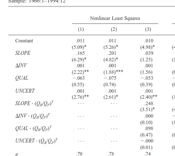
Table 2. Reduced-Form Models for the Paper-Bill Spread
Sample: 1966:1–1994:12
Nonlinear Least Squares
Two-Stage Nonlinear Least Squares
(1) (2) (3) (4) (5)
Constant .011 .011 .010 .010 .011
(5.09)* (5.26)* (4.98)* (4.08)* (4.62)*
SLOPE .165 .201 .039 .026 .036
(6.29)* (4.82)* (1.25) (1.02) (1.42)
DINV .001 .001 .001 .000 .000
(2.22)** (1.88)*** (1.56) (0.18) (0.65)
QUAL 2.063 2.075 2.053 2.100 2.179
(0.55) (0.74) (0.39) (0.85) (1.30)
UNCERT .001 .001 .001 .001 .001
(2.76)** (2.61)* (2.40)** (1.83)*** (1.74)***
CHOW 4.73* 2.65* 1.73** 0.78 1.07
HETERO 11.00* 11.09* 14.51* 9.97* 4.36**
DW 2.00 2.03 2.07 2.07 2.07
R2 .82 .82 .83 .78 .79
Notes: Numbers in parentheses are t statistics constructed with standard errors that are robust to heteroskedasticity.
EXCLUDE1 is ax2statistic to test the null hypothesis that coefficients on variables created by interacting the four explanatory variables with the 1979:10–1982:10 dummy are jointly equal to zero. EXCLUDE2 is ax2statistic used to test the null hypothesis that the coefficients on variables created by interacting the four explanatory variables with the trend value of the bill-paper quantity ratio are jointly equal to zero. CHOW is an F statistic used to test for structural stability of the model’s coefficients with the break-date set at 1979:01. HETERO is ax2statistic to test for heteroskedasticity of the model’s disturbance term linked to the trend bill-paper quantity ratio.
To directly test whether increased liquidity of the paper market was responsible for the parameter instability, the four explanatory variables (SLOPE, QUAL, DINV, and UN-CERT) were multiplied by the polynomial trend of the volume ratio and these interaction
terms were added to the model presented in column (2). The results, reported in column (3), indicate four important findings. First, thex2statistic, EXCLUDE2, allows us to reject the hypothesis that the coefficients on the interaction terms are jointly equal to zero. Second, the coefficient on SLOPEz(QB/QP)
T
instruments were the twelve monthly lags of each explanatory variable. The results, presented in column (4), were similar to those in column (3), with two exceptions. First, those in column (4) suggest that the coefficients were significantly different for the period 1979:10 –1982:10. Second, once we accounted for coefficient variation due to the mon-etary policy regime shift and rising liquidity of the paper market, the coefficients from the reduced-form model were stable.
Finally, column (5) of Table 2 allows us to examine the robustness of our findings to a different proxy for commercial paper liquidity. In particular, the model in column (5) used the 12-month moving average of the log ratio of bills to paper volumes outstanding to proxy paper liquidity. Once again, the results suggest that increased paper market liquidity caused the relationship between the paper-bill spread and its determinants to weaken.
Decomposing
The results in Table 2 generally support the hypothesis that increased liquidity of the paper market has diminished the ability of the spread to reflect information contained in its determinants. Nevertheless, the small and insignificant t statistics associated with three of the four interaction terms shown in columns (3–5) are inconsistent with this explanation. That is, if increased paper market liquidity is responsible for the diminished predictive ability of the spread, then UNCERTz(QB/QP)Tand the other interaction terms should also have positive and significant coefficients.
One possible explanation for this inconsistency is that SLOPE embodies information contained in the other explanatory variables. That is, the slope of the term structure not only gauges the stance of current monetary policy, but also reflects beliefs about future monetary policy (through expected real interest rates), expectations about future economic activity (through expected inflation premia), and interest-rate uncertainty (through risk premia) [see Estrella and Hardouvelis (1989); Ferderer (1993)]. Consequently, we may not be able to isolate the direct impact which uncertainty or other factors have on the spread because regression techniques only use variation unique to a regressor when calculating its coefficient.
To examine whether this multicollinearity problem produced the inconsistencies ob-served above, we regressed SLOPE on interest-rate uncertainty and used the residual from this regression (SLOPER) to measure the stance of monetary policy.18If the term structure contains a risk premium and becomes steeper when interest-rate uncertainty rises, this premium should not be reflected in SLOPER. The results obtained when SLOPE was replaced by SLOPER are presented in Table 3.
The results in Table 3 show that interest-rate uncertainty now has a dramatically more significant impact on the spread than it did in Table 2 across the different models. Figure 4 displays the rolling regression results using the model in column (1) of Table 3. In contrast to Figure 3, we see that interest-rate uncertainty had a positive and significant impact on the spread during the early part of the sample, and that this effect dissipated during the 1980s and early 1990s. This finding provides evidence that increased paper market liquidity over the 1980s reduced the ability of the spread to reflect interest-rate uncertainty.
The results in columns (3–5) of Table 3 confirm this visual impression. Note that the coefficient on the variable constructed by multiplying interest-rate uncertainty and the volume ratio—as well as coefficients on interaction variables created with SLOPE and
QUAL—were positive and significantly different from zero. As the ratio of bill to paper
volume fell, so do did the coefficients relating the spread to three of its four determinants. Also, the CHOW statistic suggests that the parameters were stable over the sample period once we controlled for the liquidity effect. Taken together, these findings provide additional evidence that increased liquidity of commercial paper during the 1980s reduced the sensitivity of the spread to its determinants.
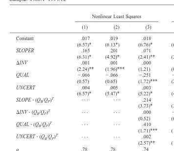
Table 3. Reduced-Form Models for the Paper-Bill Spread
Sample: 1966:1–1994:12
Nonlinear Least Squares
Two-Stage Nonlinear Least Squares
(1) (2) (3) (4) (5)
Constant .017 .019 .018 .016 .016
(6.57)* (6.13*) (6.76)* (6.17)* (6.40)*
SLOPER .165 .201 .071 .062 .048
(6.31)* (4.92)* (2.41)** (2.38)** (1.90)***
DINV .001 .001 .000 .000 .000
(2.24)** (1.96)*** (1.21) (0.07) (0.48)
QUAL 2.066 2.066 2.251 2.265 2.310
(0.57) (0.65) (1.72)*** (2.04)** (2.17)
UNCERT .004 .005 .003 .003 .003
(6.57)* (5.47)* (5.22)* (4.21)* (4.22)*
CHOW 4.72* 2.64* 1.63*** 1.07 1.04
HETERO 11.35* 11.25* 14.41* 10.67* 4.13**
DW 2.00 2.05 2.07 2.06 2.07
R2 .82 .82 .83 .78 .79
Notes: Numbers in parentheses are t statistics constructed with standard errors that are robust to heteroskedasticity.
EXCLUDE1 is ax2statistic to test the null hypothesis that coefficients on variables created by interacting the four explanatory variables with the 1979:10–1982:10 dummy are jointly equal to zero. EXCLUDE2 is ax2statistic used to test the null hypothesis that the coefficients on variables created by interacting four explanatory variables with the trend value of the bill-paper quantity ratio are jointly equal to zero. CHOW is an F statistic used to test for structural stability of the model’s coefficients with the break-date set at 1979:01. HETERO is ax2statistic to test for heteroskedasticity of the model’s disturbance term linked to the trend bill-paper quantity ratio.
V. Conclusion
Recent research has attempted to explain why the predictive power of the paper-bill spread declined during the 1980s. One explanation suggests that recent economic contractions have resulted from shocks that do not impact the paper and bill markets. Another posits that changes in paper and bill supplies unrelated to business cycle conditions have played a more dominant role in driving the spread in recent years.
This paper offers an alternative explanation. As commercial paper became more liquid during the 1980s, investors increasingly came to view paper as a close substitute for Treasury bills. As a result, shocks to the paper and bill markets had less impact on the paper-bill spread. Rather, these shocks were absorbed by proportionate yield changes in both markets. This finding can explain why the ability of the spread to predict business cycle movements declined during the 1980s.
Appendix 1
To solve for the paper-bill rate spread, first set supply equal to demand in each market and solve for the paper and bill rates. From the bill market we get:
rB5
F
1ao1bo1h
G
z$azXBS2bzXBD1hzrP1 «BS2 «BD%, (A1)
where time subscripts have been dropped for the sake of clarity. From the paper market we get:
rP5
F
1co1do1h
G
z$czXPS2dzXPD1hzrB1 «PS2 «PD%. (A2)
Now substitute equation (A1) into equation (A2) to obtain the paper rate consistent with simultaneous equilibrium in the bill and paper markets:
rP5
F
Inserting equation (A3) into equation (A1) to solve for the bill rate, we get:
rB5
F
Finally, subtract equation (A4) from equation (A3) to solve for the reduced-form for the paper-bill spread.
Appendix 2
Monthly Data1. Six-month commercial paper rate, bank discount basis, NSA (Citibase: FYCP), 1960.1–1994.12.
2. Six-month Treasury bill rate, secondary market, NSA (Citibase: FYGM6), 1960.1– 1994.12.
3. Federal funds effective rate, NSA (Citibase: FYFF), 1960.1–1994.12.
4. Ten-year Treasury bond yield, secondary market, NSA (Citibase: FYGT10), 1960.1–1994.12.
5. Aaa corporate bond yield, NSA (Citibase: FYAAAC), 1960.1–1994.12. 6. Baa corporate bond yield, NSA (Citibase: FYBAAC), 1960.1–1994.12.
8. Volume outstanding of total commercial paper (Board of Governors of the Federal Reserve System), 1966.1–1994.12.
9. Volume outstanding of Treasury bills (Treasury Bulletin), 1960.1–1994.12.
Daily Data
1. Secondary market yield on 3-month Treasury bills, discount basis (Federal Reserve
Bulletin, Table H.15, distributed by National Technical Information Services:
GFSM03), 1960.1–1994.12.
References
Amihud, Y., and Mendelson, H. Sept. 1991. Liquidity, maturity, and the yields on U.S. Treasury securities. The Journal of Finance XLVI(4):1411–1425.
Amihud, Y., and Mendelson, H. December 1986. Asset pricing and the bid-ask spread. Journal of
Financial Economics 17(2):223–249.
Bernanke, B. S. Nov./Dec. 1990. On the predictive power of interest rates and interest rate spreads.
New England Economic Review 51–68.
Bernanke, B. S., and Blinder, A. S. Sept. 1992. The federal funds rate and the channels of monetary transmission. American Economic Review 82(4):901–921.
Calomiris, C. W., Himmelberg, C. P., and Wachtel, P. 1994. Commercial paper and the business cycle: A microeconomic perspective. Mimeo. National Bureau of Economic Research. Cook, T. Q. Spring/Summer 1981. Determinants of the spread between Treasury bill rates and
private sector money market rates. Journal of Economics and Business 33:177–187.
Emery, K. M. Feb. 1996. The information content of the paper-bill spread. Journal of Economics
and Business 48(1):1–10.
Estrella, A., and Hardouvelis, G. June 1991. The term structure as a predictor of real economic activity. Journal of Finance 46(2):555–576.
Evans, P. 1984. The effects on output of money growth and interest rate volatility in the United States. Journal of Political Economy 92(2):204–222.
Ferderer, J. P. Feb. 1993. The impact of uncertainty on aggregate investment spending: An empirical analysis. Journal of Money, Credit and Banking 25(1):30–48.
Friedman, B. M., and Kuttner, K. N. Dec. 1994. Indicator properties of the paper-bill spread: Lessons from recent experience. Working Paper 94–24. Federal Reserve Bank of Chicago. Friedman, B. M., and Kuttner, K. N. 1993. Why does the paper-bill spread predict real economic
activity? In New Research in Business Cycles: Indicators and Forecasting (J. H. Stock and M. W. Watson, eds.). Chicago: University of Chicago Press, pp. 213–249.
Friedman, B. M., and Kuttner, K. N. June 1992. Money, income, prices, and interest rates. American
Economic Review 82(3):472–492.
Hafer, R., and Kutan, A. 1992. On the money-income results of Friedman and Kuttner. Working paper 92–0303. Southern Illinois University at Edwardsville.
Hamilton, J. D. 1994. Time Series Analysis. Princeton: Princeton University Press.
Hess, G. D., and Porter, R. D. August 1993. Comparing interest-rate spreads and money growth as predictors of output growth: Granger causality in the sense Granger intended. Journal of
Economics and Business 45(3):247–268.
Kamara, A. Sept. 1994. Liquidity, taxes, and short-term Treasury yields. Journal of Financial and
Quantitative Analyses 29(3):403–417.
Kramer, C. Dec. 1994. Macroeconomic seasonality and the January effect. Journal of Finance 49(5):1883–1891.
Rowe, T. D. 1986. Commercial paper. In Instruments of the Money Market (T. Q. Cook and T. D. Rowe, eds.). Richmond, VA: The Federal Reserve Bank of Richmond, 111–125.
Shen, P., and Starr, R. M. Oct. 1992. Liquidity of the Treasury market and the term structure of interest rates. Discussion paper 92–32. University of California, San Diego.
Stigum, M. 1990. The Money Market. Homewood, IL: Dow Jones Irwin.
Stock, J., and Watson, M. 1989. New indexes of coincident and leading indicators. In NBER
Macroeconomics Annual 1989 (O. J. Blanchard and S. Fischer, eds.). Cambridge, MA.: The
M.I.T. Press, 351–394.