q
The author would like to thank Jonas Fisher, Lars Hansen, Ken Judd, Martin Lettau, Per Krusell, Valerie Ramey, Tony Smith, Harold Uhlig and an anonymous referee for useful comments. *Correspondence address: Department of Economics, University of California at San Diego, La Jolla, CA 92093-0508, USA. Tel.:#1-858-534-0762; fax:#1-858-534-7040.
E-mail address:[email protected] (W.J. Den Haan). 25 (2001) 721}746
The importance of the number of di!erent
agents in a heterogeneous asset-pricing model
qWouter J. Den Haan
!
,
"
,
*
!Department of Economics, University of California at San Diego, La Jolla, CA 92093-0508, USA "National Bureau of Economic Research, Centre for Economic Policy Research, USA
Received 6 May 1998; accepted 5 April 2000
Abstract
Models with heterogeneous agents and incomplete markets often only have two types of agents to limit the computational complexity. The question arises whether equilibrium models with a realistic number of types have the same implications as models with a small number of types. In the asset-pricing model considered in this paper, several properties depend crucially on the number of types. For example, in the economy with only two types interest rates respond to&idiosyncratic'income shocks which makes it easier to smooth consumption. Moreover these e!ects can be so strong that it is possible that a relaxation of the borrowing constraintreducesan agent's utility. Average interest rates on the other hand are not very sensitive to the number of types. ( 2001 Elsevier Science B.V. All rights reserved.
JEL classixcation: E21; E43; C61
Keywords: Dynamic model; Large state space model
1For example, Judd et al. (1998) and Krusell and Smith (1998) consider heterogeneous pre-ferences.
2Cf. Weil (1992).
3Examples are Heaton and Lucas (1992, 1996), Lucas (1994), Marcet and Singleton (1999), Telmer (1993), and Zhang (2000). Alternatively, it is assumed that there is no aggregate uncertainty and a continuum of agents. In this case asset prices are constant over time. See, for example, Aiyagari (1994) and Aiyagari and Gertler (1991).
4Cf. Den Haan (1996, 1997), Gaspar and Judd (1997), Krusell and Smith (1997, 1998), and Rios-Rull (1996). See Rios-Rull (1997) for an overview.
1. Introduction
Dynamic equilibrium models with heterogeneous agents and incomplete markets have become popular tools in the macro asset-pricing literature. Het-erogeneity usually arises because an agent's income is a!ected not only by aggregate but also by idiosyncratic income shocks, but other forms of hetero-geneity have also been considered.1These models have been shown to be an improvement over standard representative agent models in several dimensions. For example, they provide an explanation for the low level of real interest rates observed in the US data.2The reason is that the presence of idiosyncratic risk provides an additional incentive to save which lowers real interest rates. Many models analyzed in the literature have only two di!erent types of agents.3In these models, individual speci"c shocks are not truly idiosyncratic since all agents of the same type receive the same shock. One could interpret an agent's idiosyncratic income shock in an economy with two types as a sector-speci"c shock. This has two disadvantages. First, although moral hazard can be used to explain why contracts that are contingent on an individual's income realization do not exist, it cannot be used to rule out contracts contingent on the perfor-mance of the sector. The second disadvantage of interpreting the idiosyncratic shocks as sector speci"c shocks is that the variability of the average income in a sector is a lot smaller than the variability of individual income. Without having a substantial amount of idiosyncratic uncertainty, however, the predic-tions of heterogeneous agent models are not that di!erent from models with a continuum of agents.
In this paper, I analyze an in"nite-horizon equilibrium model of the short-term interest rate similar to that used in the literature except that it has a continuum of types instead of two types. Markets are assumed to be incom-plete, but agents can smooth their consumption by trading in risk-free bonds. For the parameter values considered in this paper, average interest rates in the model with a large number of di!erent agents are very similar to average interest rates in the corresponding model with only two types of agents. In the presence of borrowing constraints, the model with a continuum of types, thus, also predicts low average real interest rates. Several other properties of the model studied in this paper, however, depend crucially on the number of types.
The"rst important di!erence between the two models is that the amount of
5In this paper, stationary variables are denoted by small characters and non-stationary variables are denoted by capital characters.
6Wang (1995) shows that contracts contingent on the realization of the shock are possible when multi-period contracts are enforceable.
The organization of this paper is as follows. In the next section, an in" nite-horizon endowment economy with incomplete markets will be discussed. In Section 3, I analyze the properties of the economy with a continuum of types and those of the economy with two types. The last section concludes.
2. An equilibrium model with heterogeneous agents
In this section, I develop an in"nite horizon model of the short-term interest rate similar to the models in Deaton (1991) and Pischke (1995). In contrast to Deaton (1991) and Pischke (1995), the interest rate is not constant but varies to ensure that the bond market is in equilibrium. In Section 2.1, I discuss the optimization problem of the individual agent. In Section 2.2, I discuss the equilibrium condition, and in Section 2.3, I discuss the parameter values used.
2.1. The individual agent's problem
Ex ante agents are exactly the same, but ex post di!er due to the presence of idiosyncratic shocks. In particular, the endowment of agentirelative to the per capita endowment,yit, can take on a low value,yL, and a high value, yH. The (gross) growth rate of the per capita endowment,a
t"At/At~1, can also take on
a low (or recession) value,aR, and a high (or boom) value,aB.5Both processes are assumed to be"rst-order Markov processes.
In an economy in which all shocks are observed without costs, it would be optimal to write contracts contingent on the realization of the idiosyncratic shock. If it is impossible for the lender to verify the realization of the borrowers income, the borrower would always report that he received the lowest possible realization. In this case, the optimal one-period contract is a bond with a"xed payment.6It is assumed here that agents can only smooth their consumption by trading in a one-period risk-free bond. Markets are, thus, incomplete.
Agenti's maximization problem is as follows:
max
MCit,BitN= t/0
= + t/0
btC1~t c!1
1!c
s.t. Cit#q
7See Ja!ee and Stiglitz (1990, Section 5.3) and the references therein.
8See, for example, Bernanke et al. (1996).
whereCitis the amount of consumption of agentiin periodt,Bit is the demand for one-period bonds that pay one unit of the consumption commodity in the next period,q
tis the price of this one-period bond, andBi~1is given. The agent
takes the bond price as given. The interest rate,r
t, is de"ned as (1!qt)/qt.
The question arises whether a lender would want to restrict the amount he is willing to lend to a borrower. It would make sense to limit the amount of debt by the net present value of the borrower's endowment stream. In this economy, in which agents live and receive an endowment stream for ever, this constraint is unlikely to seriously restrict the demand for loans. In reality, however, con-sumers and "rms do seem to face borrowing constraints.7 More restrictive borrowing constraints arise in our model if one makes the assumption that the borrower faces limited costs of defaulting on the loan. Suppose that the default costs are equal toBMt. In this case, borrowers will default whenever!B
t5BMt.
This, of course, implies that the lender will never lend more thanBM t. I assume thatBMt (scaled by the per capita endowment) is a constant. Thus, the following borrowing constraint is added to the maximization problem:
Bit5!b1A
t. (2)
Note thatBitincludes the interest payments on the bond. LetBIit("q
tBit) denote
the amount of savings net of interest payments. Then Eq. (2) can be rewritten as follows:
BIit5! b1At 1#r
t
. (3)
Eq. (3) is a typical formulation of a borrowing constraint.8It has the property that the maximum amount an agent can borrow is decreasing with the interest rate. The"rst-order conditions for the maximization problem of the agent are the two-part Kuhn}Tucker conditions:
q
t[Cit]~c5bEt[Cit`1]~c and
(Bit#b1A
t)(qt[Cit]~c!bEt[Cit`1]~c)"0.
(4)
The equations of this model can easily be transformed to a system of equations that contains only stationary variables. To see this, de"nez
9See Judd et al. (1998) for a discussion on state variables in this type of model.
Two di!erent versions of the model are considered. In both versions there are a continuum of agents with unit mass. In the "rst version, the idiosyncratic draws, yit, are distributed independently across agents and across time. In the second version, there are only two types of agents and each agent always receive the same realization of the idiosyncratic shock as the other agents of the same type. Note that in the economy with two typesy1t andy2t are perfectly negatively correlated sincey1t#y2
t"2. This restriction will be discussed in detail in the
next section.
LetFLt andFHt be the cumulative distribution function of the cross-sectional beginning-of-period bond holdings of the agents who receive the low-income shock and the high-income shock, respectively. In the economy with only two types, all agents who receive the low realization for the idiosyncratic shock have the same amount of beginning-of-period bond holdings since they all have the same history of idiosyncratic shocks. The same is true for the agents who receive the high value. Consequently, dFL and dFH have mass at only one level of b
t~1 in the economy with two agents. In contrast, in the economy with
a continuum of types, there will be a wide variety of bond holdings at each point in time.
The state variables of agentiarebit~1,yit, and the aggregate state variablesa6
t.
Agent i's demand for bond holdings is assumed to be a function of the state variables.9The equilibrium condition for the bond market is given by
P
=In the economy with two types, information about the idiosyncratic shock and bond holdings of one type disclose the corresponding values of the other type. The set of aggregate state variables (a6
t) is, thus, equal to the growth rate of the
aggregate endowment,a
t. In the economy with a continuum of di!erent agents,
the aggregate state variables area
t, the cross-sectional distribution of the bond
holdings of the low-income agents, and the cross-sectional distribution of the bond holdings of the high-income agents. A solution to the model, in this case, consists of a consumption function,c(b
t~1,yt,at,FLt,FHt), an investment
func-tion, b(b
t~1,yt,at,FLt,FHt), a bond price function, q(at,FLt,FHt), and the
func-tionals FL(a
10The reported values are two times those reported in Heaton and Lucas (1996) since Heaton and Lucas (1996) de"ney
tas the share of the aggregate endowment one agent receives, while this paper de"nesy
tas the endowment relative to the per capita endowment to ensure that the de"nition also makes sense in the case with a continuum of types.
law of motion ofFL
t andFHt, respectively. The only reason why the current value
ofa
tis an argument of the transition functionals is that the beginning-of-period
bond holdings are scaled relative to the per capita endowment. For example, suppose that in periodt!1 an agent borrows the maximum amount b1 A
t~1.
Thus, b
t~1"!b1. This means that in period t, beginning-of-period bond
holdings, relative to the aggregate endowment, are equal to!b1/a t.
Several papers in the literature discuss the existence of equilibrium. Existence of equilibrium with borrowing constraints in an economy like ours but with
a"nite number of agents is discussed in Magill and Quinzii (1994). Den Haan
(1997) compares the numerical solution to the model with a continuum of agents with the simulated results of an economy with 100,000 agents and"nds that the results are very similar. This suggests that there are no di!erences between an economy with a continuum of agents and an economy with a large but"nite number of agents. Related papers are Du$e et al. (1994), Levine (1989), and Levine and Zame (1993).
2.3. Parametervalues
The time period in the model corresponds to a year and the discount rate is set equal to 0.965. Asset prices and consumption behavior crucially depend on the assumed values for the degree of relative risk aversion,c, and the borrowing constraint parameter,b1. I, therefore, consider values forcequal to 1, 3, and 5 and values forb1 ranging from 0.2 to 2.0.
The parameter values of the stochastic driving processes for A
t andyit are
identical to those used in Heaton and Lucas (1996). Heaton and Lucas (1996) obtained estimates for these processes using the income series from the Panel Studies of Income Dynamics (PSID) under the assumption that both processes are two-state"rst-order Markov processes. The two values for the idiosyncratic shock,10y
t, are 0.7544 and 1.2456 and the two values for the aggregate (gross)
growth rate,a
t, are 0.9904 and 1.0470. The probability of receiving in this period
the same idiosyncratic shock as was received in the last period is equal to 0.7412 and the probability of receiving the same aggregate shock is equal to 0.5473.
Note that the time-series speci"cations for A
t and yit are the same in both
11Since the amount of aggregate risk is small relative to the amount of idiosyncratic risk this example is not that di!erent from the actual model used.
idiosyncratic uncertainty as well as the empirical value for the amount of aggregate uncertainty imposes restrictions on the joint distribution of>1
t and
>2
t in the economy with two agents. To understand this consider the case where
there is no aggregate uncertainty andA
t"A1 in every period.11To ensure that
A
t"A1, it must be the case in the economy with two agents that>1t and>2t are
perfectly negatively correlated. In contrast, in the economy with a continuum of agents >it and >jt can be independent for iOj. A law of large numbers guarantees thatA
t"A1. If one would assume that>1t and>2t are independent in
the economy with only two agents as well then the amount of aggregate uncertainty would depend on the number agents. In this case, the properties of the model would depend on the number of agents even when markets are complete because the amount of aggregate uncertainty depends on the number of agents.
3. The properties of diverse and less-diverse economies
In this section, I analyze the properties of the two equilibrium models described in Section 2. Agents in the two economies face exactly the same amount of idiosyncratic and aggregate endowment risk. The joint time-series properties di!er considerably, however. In the economy with two types, an agent's idiosyncratic shock is perfectly positively correlated with the shocks of half of the population. In the economy with a continuum of di!erent agents, an agent's idiosyncratic shock is distributed as an independent random variable. In Section 3.1, I analyze the time-series properties of the interest rate. In Section 3.2, I analyze the time-series properties of consumption and bond purchases in the two economies. In Section 3.3, I analyze the ability to insure against idiosyncratic shocks in the two economies.
3.1. Interest rates in diverse and less-diverse economies
Fig. 1. Cross-sectional dispersion and the interest rate. This "gure plots the interest rate as a function of the low-income agent's beginning-of-period debt level in the economy with two types. As the debt of the low-income agent increases, the amount of cross-sectional dispersion increases. The borrowing constraint parameter is equal to 1.4 and the parameter of relative risk-aversion is equal to 3. The graph is drawn for the low realization of the aggregate growth rate.
12Carroll and Kimball (1996) showed that this property holds in intertemporal optimization models under very general conditions.
3.1.1. The amount of cross-sectional dispersion and the interest rate
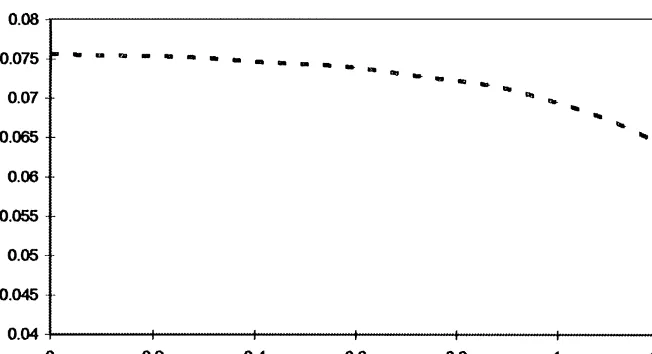
Fig. 2. The average bond price in diverse and less diverse economies. This graph plots the average bond price as a function of the borrowing constraint parameter. The borrowing constraint para-meter indicates the maximum amount an agent is allowed to borrow relative to the per capita endowment. The parameter of relative risk aversion is equal to one (three) in the case of low (high) risk-aversion. The other parameter values are reported in Section 2.3. Population moments are approximated using the moments calculated with a simulated draw of 100,000 observations.
consider the extreme case when there is no cross-sectional dispersion. In this case, the marginal propensities to save are equal for all agents and a marginal wealth transfer would increase the amount of dispersion but would have no e!ect on the interest rate.
The e!ects are magni"ed in the presence of borrowing constraints since borrowing constraints reduce the marginal propensity to save of the less wealthy even further. When a poor agent has reached his debt limit, a wealth transfer from this agent to a wealthier agent requires a large drop in the interest rate since the new interest rate has to be such that the wealthier agent is willing to consume the total wealth transfer. This explains the kink in Fig. 1. At the kink, the poor agent has reached his borrowing constraint and the slope of the function sharply decreases.
3.1.2. Time-series behavior of the interest rate
13Jensen's inequality implies that the di!erences are smaller for average interest rates than for average bond prices because the interest rate is a concave function of the bond price.
14Examples are Heaton and Lucas (1996), Lucas (1994), and Telmer (1993).
15Not shown in the graph is the result that when the borrowing constraint parameter is equal to 0.2 and the parameter of relative risk aversion is equal to"ve, then the di!erence in average bond prices is equal to 2.9 percentage points.
16Note that this is not a formal argument. One reason is that characterizing the amount of cross-sectional dispersion is much more complex in the economy with a continuum of agents. For example, in the economy with two types the amount of beginning-of-period bond holdings of the low-income agents completely describes the amount of cross-sectional dispersion. In the economy with a continuum of types this is not the case. Also, even if the same measure of cross-sectional dispersion is used, the relationship between the interest rate and the amount of cross-sectional dispersion does not have to be the same in the two types of economies. Finally, the average amount of cross-sectional dispersion may di!er across the two types of economies.
of the borrowing constraint parameter. I choose to plot the average bond price because the di!erences are bigger for the bond price than for the interest rate.13
Nevertheless, the results are remarkably similar for most parameter values. This is good news for several papers in the asset-pricing literature that mainly focused on average returns.14 As documented in the graph, some di!erences can be found when the borrowing constraint parameter is low and the parameter of relative risk aversion is high. When the borrowing constraint parameter is equal to 0.2 and the parameter of relative risk aversion is equal to three, for example, then the average bond price in the economy with two types is 1.4% higher than the average bond price in the economy with a continuum of types.15For many purposes these di!erences are of little importance. When one wants to know the e!ect of a change in the borrowing constraint parameter from 0.2 to 2.0, for example, then the economy with two types predicts a decrease in the average bond price of 13.3% and the economy with a continuum of types predicts a decrease of 12.0%.
The results from the last subsection provide an intuitive explanation for the
"nding that the average interest rate (bond price) is lower (higher) in the
economy with two types. Since the interest rate is a concave function of the amount of cross-sectional dispersion and the amount of cross-sectional disper-sion is considerably more volatile in economies with two types of agents, Jensen's inequality suggests that the average interest rate should be lower in the economy with economy with two types.16
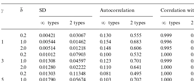
Table 1 documents the di!erences across the two types of economies for the following time series statistics of the interest rate: the standard deviation, the
"rst-order autocorrelation coe$cient, and the correlation with the growth rate
Table 1
Time-series behavior of the interest rate!
c b1 SD Autocorrelation Correlation witha
t
Rtypes 2 types Rtypes 2 types Rtypes 2 types
0.2 0.00421 0.03067 0.130 0.555 0.999 0.132
1 1.0 0.00544 0.01462 0.154 0.683 0.996 0.291
2.0 0.00514 0.01218 0.148 0.606 0.995 0.347
0.2 0.01012 0.07903 0.100 0.532 1.000 0.118
3 1.0 0.01308 0.04597 0.123 0.701 0.999 0.261
2.0 0.01280 0.02222 0.110 0.641 1.000 0.451
0.2 0.01303 0.11348 0.081 0.495 1.000 0.116
5 1.0 0.01790 0.05674 0.103 0.702 1.000 0.281
2.0 0.01956 0.02913 0.097 0.606 1.000 0.527
!Note: This table reports time-series statistics of the interest rate on a one-period bond.cdenotes the parameter of relative risk aversion andb1 indicates the amount the agent is allowed to borrow relative to the per capita endowment. The other parameter values are reported in Section 2.3. Population moments are approximated using the sample moments of a simulated draw of 100,000 observations.
deviation of interest rates across the two types of economies. This can be explained by the large di!erences in the volatility of the amount of cross-sectional dispersion across the two types of economies. Heaton and Lucas (1996) report that in models with two types of agents it is not possible to"t the equity premium without bond returns being excessively volatile. Heaton and Lucas (1996) report a standard deviation for US bond returns equal to 0.026. As documented in Table 1, for values ofcandb1 that produce low average interest rates (i.e. high values ofcand low values ofb1), the volatility in the economy with two types is indeed much higher than what is observed in the data. In the corresponding economies with a continuum of agents, however, the volatility of interest rates is never larger than what is observed in the data.
Second, the autocorrelation of the interest rate is much higher and much closer to the observed autocorrelation in the economy with two types. The reason is that in this type of economy the interest rate is in#uenced by realiz-ations of the idiosyncratic shock which are much more persistent than shocks to the aggregate growth rate. Of course, this does not seem like a plausible explanation for the observed persistence.
Note that in the presence of complete markets, the interest rates would be exactly the same in both types of economies. Consistent with this is the observation that the di!erences across the two types of economies become smaller when the borrowing constraint parameter increases, that is, when the
"nancial frictions become smaller.
3.2. Consumption and bond holdings
In this section, I analyze the time-series behavior of consumption and bond purchases in the economy with two types and the behavior of these variables in the economy with a continuum of types. The consumption variable that I focus on is the percentage change in individual consumption,*lnC
t"*ln (ctAt).
Since bond purchases can take on negative values and values close to zero, it does not make sense to use the percentage change. To study the behavior of bond purchases I, therefore, focus on the amount of bonds purchased relative to the per capita endowment,b
t"Bt/At. This variable has the disadvantage that
its unconditional covariance with any aggregate variable is by construction equal to zero because agents are ex ante identical. The statistics considered for the consumption variable are the standard deviation, the correlation with the individual endowment growth rate, the correlation with the aggregate consumption growth rate, and the correlation with the interest rate. The statistics considered for the bond purchases are the standard deviation, the
"rst-order autocorrelation coe$cient, the correlation with the idiosyncratic
endowment shock, and the fraction of times the agents is at the constraint. The results are reported in Tables 2 and 3 for consumption and bond purchases, respectively.
The following observations can be made. First, in both types of economies, the correlation between individual consumption growth and income growth decreases and the correlation between individual and aggregate consumption growth increases when the borrowing constraint parameter increases. Results not reported here show that the amount of serial correlation in consumption growth reduces when the borrowing constraint parameter increases. These
"ndings, thus, document that as"nancial frictions weaken agents are better able
Table 2
Time-series behavior of individual consumption growth!
c b1 SD Correlation with*ln (>
t) Correlation withat Correlation withrt
Rtypes 2 types Rtypes 2 types Rtypes 2 types Rtypes 2 types
0.2 0.140 0.135 0.888 0.924 0.198 0.206 0.198 0.057
1 1.0 0.070 0.065 0.724 0.783 0.404 0.439 0.402 0.152
2.0 0.051 0.045 0.646 0.687 0.540 0.626 0.537 0.234
0.2 0.131 0.122 0.891 0.927 0.211 0.226 0.211 0.055
3 1.0 0.071 0.057 0.761 0.811 0.397 0.487 0.396 0.139
2.0 0.056 0.047 0.713 0.736 0.490 0.597 0.490 0.284
!Note: This table reports the time-series statistics for the percentage change in individual consumption growth,*lnC
t. The variable*ln>tdenotes the
percentage change in the individual endowment.a
tis the growth rate of aggregate endowment which equals the growth rate of aggregate consumption.
r
tis the interest rate.cdenotes the parameter of relative risk aversion andb1 indicates the amount the agent is allowed to borrow relative to the per capita
endowment. The other parameter values are reported in Section 2.3. Population moments are approximated using the sample moments of a simulated draw of 100,000 observations.
W.J.
Den
Haan
/
Journal
of
Economic
Dynamics
&
Control
25
(2001)
721
}
Table 3
Time-series behavior of individual bond purchases!
c b1 SD Autocorrelation Correlation withy
t Fraction at constraint
Rtypes 2 types Rtypes 2 types Rtypes 2 types Rtypes 2 types
0.2 0.198 0.166 0.844 0.788 0.794 0.887 0.312 0.294
1 1.0 0.775 0.636 0.967 0.954 0.456 0.532 0.085 0.081
2.0 1.349 1.142 0.986 0.981 0.303 0.353 0.021 0.038
0.2 0.190 0.166 0.831 0.781 0.823 0.893 0.309 0.298
3 1.0 0.747 0.660 0.966 0.956 0.466 0.515 0.068 0.107
2.0 1.319 1.192 0.986 0.983 0.305 0.334 0.016 0.052
!Note: This table reports the time-series statistic for the bond purchases relative to the current per capita endowment,b
t. The variableytdenotes the
agent's endowment relative to the per capita endowment.cdenotes the parameter of relative risk aversion andb1 indicates the amount the agent is allowed to borrow relative to the per capita endowment. The other parameter values are reported in Section 2.3. Population moments are approximated using the sample moments of a simulated draw of 100,000 observations.
Den
Haan
/
Journal
of
Economic
Dynamics
&
Control
25
(2001)
721
}
746
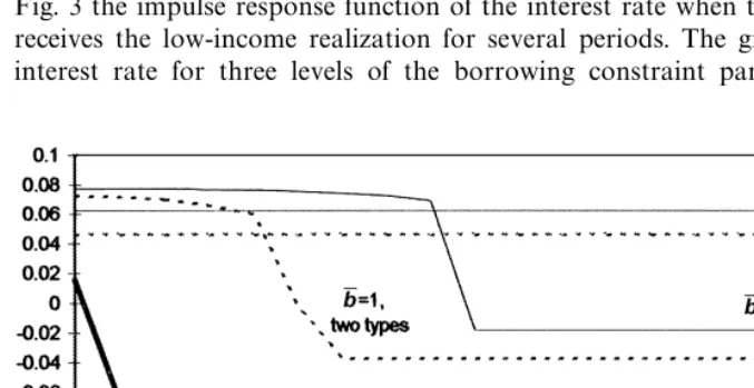
Fig. 3. The response of the interest rate to idiosyncratic shocks. This graph plots the realization of the interest rate in the economy with two types when the agent receives the low-income realization for several periods. The straight line drawn with the same style indicates the interest rate in the corresponding economy with a continuum of types. The parameter of risk aversion is equal to three and the aggregate growth rate is always equal to the low value. The parameterb1 indicates the amount an agent is allowed to borrow relative to the per capita endowment. The values of the other parameters are reported in Section 2.3.
3.3. Insurance against idiosyncratic risk
A crucial feature of the economy with two types is that the interest rate drops when an agent receives the low realization for several periods because of the increase in cross-sectional dispersion. This works like a transfer from the rich agents (the lender) to the poor agents (the borrower) and suggests that agents in economies with only two types are better o! than agents in economies with a continuum of types. There is another e!ect, however, that makes it harder to smooth consumption in economies with two types. It is harder to smooth consumption in an economy with two types because an agent will not lend to another agent of the same type and can never lend more than the agent of the other type is allowed to borrow. This will prevent him from building up a large bu!er stock during good times. Agents in an economy with a continuum of types can lend to a wide variety of di!erent agents and at times accumulate assets well in excess over the maximum amount that is possible in an economy with two types.
17It is assumed that the economy has been in a recession for several periods so that there are no more dynamic adjustments in the interest rate in the economy with a continuum of agents.
parameter of relative risk aversion equal to three. The agents in the economy with two types start out with zero bond holdings, and without loss of generality, I consider the case where the economy is in a recession. The graph also plots the interest rate in the economy with a continuum of types that, of course, does not respond to the realizations of an individual's income shock.17 Consider the initial period in the two models. Since the initial levels of bond holdings are equal to zero in the economy with two types, there is little cross-sectional dispersion when the agent receives his "rst low-income realization. In the economy with a continuum of types there always is a certain amount of dispersion. Initially, therefore, the interest rate is lower in the economy with a continuum of types, since higher cross-sectional dispersion corresponds to lower interest rates. When the agent receives additional negative shocks, the amount of cross-sectional dispersion in the economy with a continuum of types is not a!ected but increases in the economy with two types. As documented in the graph, this causes the interest rate to drop. Quantitatively, these e!ects are enormous. When the agent reaches his constraint in the economy with two types, then the interest rate is equal to!15%,!3.7%, and!1.8%, for values of the borrowing constraint parameter equal to 0.2, 1.0, and 2.0, respectively. These negative interest rates imply that the agent consumes more than his income level when he reaches the constraint. Not bad, to live in a world in which changes in the interest rate provide this kind of insurance!
The graph does not reveal the ability of an agent in the economy with a continuum of types to accumulate more assets during good times. The next
two"gures reveal both this e!ect and the interest rate e!ect discussed above. In
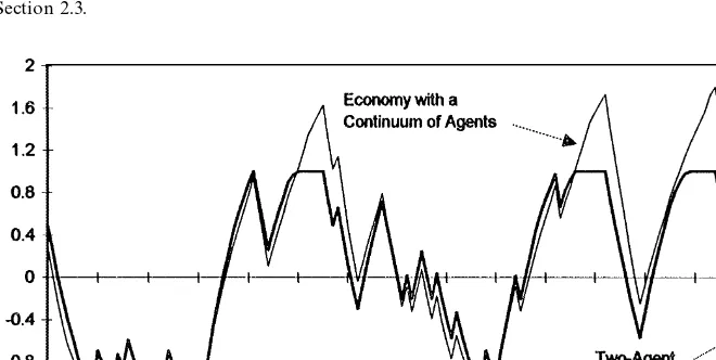
Fig. 4. A realization for individual consumption. This graph plots the consumption levels relative to the per capita endowment for the indicated economy. The parameter of relative risk aversion and the borrowing constraint parameter are equal to one. The values of the other parameters are reported in Section 2.3.
Fig. 5. A realization for individual savings. This graph plots the savings decision relative to the per capita endowment for the indicated economy. The parameter of relative risk aversion and the borrowing constraint parameter are equal to one. The values of the other parameters are reported in Section 2.3.
Table 4
Welfare comparisons!
A. Permanent percentage increase of consumption to become as well o!as in complete markets economy
c"1 c"3 c"5
b1 Rtypes 2 types Rtypes 2 types Rtypes 2 types
0.2 1.70 1.71 4.43 4.16 6.10 5.09
1.0 0.70 0.71 2.13 1.98 3.45 2.95
2.0 0.46 0.36 1.68 1.66 3.20 3.68
B. Permanent percentage increase of consumption to become as well o!as in the economy with two types
b1 c"1 c"3 c"5
0.2 !0.01 0.27 0.96
1.0 !0.01 0.15 0.49
2.0 0.07 0.02 !0.45
!Note: Panel A reports the permanent increase in consumption that is required to make an agent in the indicated economy as well o!as an agent in the complete markets economy. Panel B reports the permanent change in consumption that is required to make an agent in the economy with a continuum of types as well o!as an agent in the economy with two types. To calculate the (unconditional) expected discounted utility the average of the actual discounted utility levels across 50,000 replications of 250 observations is used. In each replication, the initial conditions are drawn from the ergodic distribution.cis the parameter of relative risk aversion andb1 indicates the amount an agent is allowed to borrow relative to the per capita endowment. The values of the other parameters are reported in Section 2.3.
18The discounted utility of consumption in periods 251 and higher is so small that ignoring it does not a!ect the results.
consumption shows that the agent in the economy with a continuum of types is better able to smooth his consumption in the periods after which he has built up a large bu!er stock of savings.
19This paper, thus, provides the"rst politically correct argument against diversity.
economies relative to the complete markets economies. In particular, it reports the permanent percentage increase in consumption that would make the agents in the incomplete markets economies as well o!as the agents in the complete markets economy. The table documents that agents in the incomplete markets economies are substantially worse o! at the lower levels of the borrowing constraint parameters, especially for the higher levels of risk aversion.
Panel B reports the permanent percentage change in consumption that would make an agent in the economy with a continuum of types as well o!as an agent in the economy with two types. For most parameter values, this number is positive, which means that an agent is better o!in an economy with only two di!erent types of agents.19 In these cases, the interest rate e!ects are more important than the ability to accumulate high levels of assets. The results are quantitatively important for some parameter values. When the parameter of relative risk aversion is equal to "ve (three) and the borrowing constraint parameter is equal to 0.2, for example, then an agent in the economy with two types is willing to permanently reduce his consumption by 0.96 (0.27)% to avoid being in an economy with a continuum of types. An important exception is the case when the parameter of risk aversion is equal to"ve and the borrowing constraint parameter is equal to two. In this case, the agent is better o!in the economy with a continuum of types.
One more interesting observation can be made about the economy with two types. As documented in Panel A, when the parameter of risk aversion is equal
to"ve, then an increase in the borrowing constraint parameter from 0.2 to 1.0
makes the agent better o!, but a further increase leads to a decrease in the agent's expected utility. The reason is that for higher levels of risk-aversion, the interest rate e!ects are so helpful in smoothing consumption that being in an economy with a higher borrowing constraint parameter does not make you necessarily better o!. To understand this result, I plot in Fig. 6 the impulse response function of consumption (relative to the per capita endowment) when the agent receives the low-income realization for several periods.
The graph makes clear how it can be possible that an agent's expected utility is higher when the borrowing constraint parameter is equal to 1.0 than when the borrowing constraint parameter is equal to 0.2 or 2.0. Note that the agent's consumption whenb1"1.0 is never far below the maximum consumption level for the other two values of b1. But when b1"0.2 an agent's consumption is considerably lower than the alternatives if he has been hit a few times by a low realization. Similarly, when b1"2.0 an agent's consumption is considerably lower when he has been hit by a large string of low realizations.
Fig. 6. The response of consumption to a series of negative idiosyncratic shocks. This graph plots the realization of consumption in the economy with two types when the agent receives the low-income realization for several periods. The parameter b1 indicates the amount an agent is allowed to borrow relative to the per capita endowment. The parameter of risk aversion is equal to
"ve and the aggregate growth rate is always set at the low value.
negative. One might think that the agent that is allowed to borrow less would
bene"t less from the negative interest rates. In fact, the opposite is true and the
agents are consuming more when they face tighter borrowing constraints. The reason is that the interest rate drops to a much more negative value in economies with tight borrowing constraints.
4. Concluding comments
In this paper, I analyze the properties of an asset-pricing model with a con-tinuum of types and the properties of the corresponding model with two types. Besides the number of types, the two models are exactly identical. In particular, the univariate time-series speci"cations of the individual and aggregate endow-ment are the same in the two models.
The following properties for the time-series behavior of interest rates are found.
f Average interest rates are remarkably similar for the parameters considered
f Interest rates are much more volatile in economies with only two types
because an important part of the #uctuations in interest rates is due to idiosyncratic shocks. Unlike economies with two types, economies with a continuum of types can have low real interest rates without having excess-ively volatile bond returns.
The di!erent time-series behavior of interest rates causes the behavior of consumption and bond purchases to di!er as well. The following di!erences are found.
f In an economy with two types, each agent can never invest more than the
agents of the other types are allowed to borrow. In an economy with a continuum of types, equilibrium on the bond market does not create such a constraint. Consequently, in the economy with a continuum of types, agents accumulate during good times assets well in excess of the amount they are allowed to borrow. This makes it easier to smooth consumption.
f There is also a reason why it is easier to smooth consumption in the economy
with two types. If, in an economy with two types, the same agent is hit by a series of negative &idiosyncratic' shocks, the amount of cross-sectional dispersion increases which leads to a drop in the interest rate. The reduction in the interest rate works like a transfer from the rich agents (the lenders) to the poor agents (the borrowers). For most parameter values, this e!ect is more important and the agent's expected utility is higher in economies with only two types.
f For higher values of the parameter of relative risk aversion these interest rate
e!ects become so strong that the e!ect of"nancial frictions on agent's welfare has a di!erent sign in the two types of economies. In economies with a continuum of types, an agent's welfare is always increasing when the maximum amount he is allowed to borrow increases. In the economy with two types, however, there are parameter values for which an agent's welfare is
decreasingwhen the borrowing constraint is relaxed.
Appendix A. The solution algorithm
a large (but"nite) number of state variables without reducing the dimension of the set of state variables is Gaspar and Judd (1997).
In the model, the bond price at periodt is a function of a
t and the
cross-sectional distribution of bond holdings. A key feature of the proposed algorithm is to approximate the cross-sectional distribution of wealth and income holdings at period t using an (M]1) vector, /
t, containing moments of the
cross-sectional distribution. To approximate the bond price function I, therefore, use the functionH(a
t,/t;d
H
), wheredH
is a vector of parameters andH()) is chosen
from a class of functions that can approximate any function arbitrarily well. Similarly, I use the functionU(a
t`1,at,/t;d
U
) to approximate the transition law of/
t. Since/tis a vector,U()) is a vector-valued function. Solving the individual
problem requires approximating one more function. I approximate the condi-tional expectation, E
t[cit`1]~c, and denote the approximating function by
W(yit,bit~1,a
t,/t;dW).
For a particular functional form forH()),U()), andW()), the algorithm solves
for the parameter valuesdU , dH
, anddW
with the following iteration scheme:
Step1: Given parameter values fordU anddH
, solve the individual's problem, that is, obtain parameter values for dW
. The number of state variables for this problem is equal to six. Other than the somewhat high number of state variables, this is a straightforward numerical problem.
Step 2: Given the decision rules for the individuals, solve the aggregate problem, that is, obtain parameter values fordU
anddH
. Since the cross-sectional density is assumed to belong to a certain class of densities, knowing the moments is the same as knowing the density. At each point in the state space one can use numerical integration techniques and the individual policy functions derived in step 1 to calculate the equilibrium interest rate and the moments of next period's cross-sectional distribution. A simple projection is used to calcu-late the values fordUanddH. If these parameter values are&close'to the ones used to solve the individuals problem in step 1, then the algorithm has converged. If not, one has to repeat steps 1 and 2.
In this paper, I use the"rst two moments of the bond holdings of the agents who receive the low-income shock and the "rst two moments of the bond holdings of the agents who receive the high-income shock to approximate the cross-sectional distributions. In this caseMequals 3 since the means of the two cross-sectional distributions add up to zero. Other choices of the numerical solution procedure are the same as those for EXP2Q500 described in Table 2 of Den Haan (1997).
The numerical procedure to solve the model with only two types is relatively straightforward and requires only obtaining a numerical approximation
WH(yit,bit~1,a
t;dWH) to Et[cit`1]~c. Note that /t is not an argument of WH())
because the variables yit, bit~1, and a
t completely describe the state of the
economy at period t. The parameter values for dWHare obtained in a manner
similar to the procedure used to solvedW
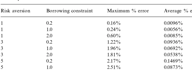
Table 5
Euler equation errors!
Risk aversion Borrowing constraint Maximum % error Average % error
1 0.2 0.16% 0.0096%
1 1.0 0.24% 0.0056%
1 2.0 0.60% 0.0085%
3 0.2 1.22% 0.0936%
3 1.0 1.96% 0.0692%
3 2.0 1.81% 0.0538%
5 0.2 2.17% 0.1469%
5 1.0 2.51% 0.0873%
5 2.0 4.19% 0.0629%
!Note: This table reports for di!erent parameter values the maximum and the average Euler equation errors calculated over a grid of 1000 beginning-of-period bond holdings for each of the four exogenous states.
types. The only di!erence is that now the bond price is solved simultaneously using a nonlinear equation solver by imposing that the demand for bonds of the two types of agents adds up to zero. As in Den Haan (1997) orthogonal Chebyshev polynomials are used for the approximating function. Here a 49th-order polynomial is used.
Accuracy of the solution procedure used to solve the model with a continuum of types is discussed in Den Haan (1997). Since solving the model with two types requires only obtaining an approximation to the conditional expectation one can use the Euler equation errors calculated over a "ne grid to assess the accuracy of the solution procedure. These errors are reported in Table 5 and are calculated as follows.
1. Using the approximation to the conditional expectations for the two agents, I calculate the equilibrium bond price and the consumption level for agent 1. 2. I recalculate the conditional expectations for the two agents. To calculate the current-period savings decision, tomorrow's bond price, and tomorrow's consumption levels I use the obtained numerical approximation.
3. Using the recalculated conditions expectations I resolve the equilibrium bond price and the consumption level for agent 1.
4. I calculate the percentage (absolute) di!erence between the consumption levels obtained in steps 1 and 3.
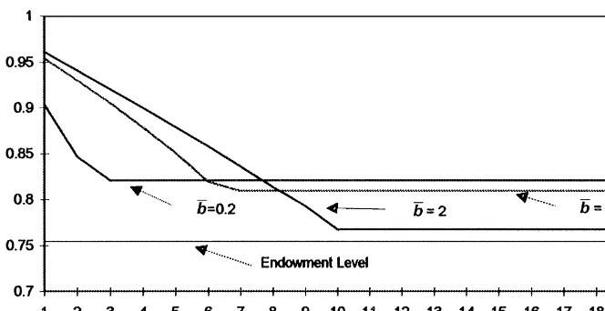
Fig. 7. The accuracy of the numerical solution for the consumption function. This graph plots the numerical solution of the consumption function and the consumption level that corresponds to the conditional expectation that is recalculated at the indicated level of beginning-of-period bond holdings. The parameter of relative risk aversion is equal to 5 and the borrowing constraint parameter is equal to 2.
one corresponding to the numerical solution. The one with tiny blips corre-sponds to the consumption level based on the conditional expectation that is recalculated at the indicated beginning-of-period bond holdings. Since these blips are unlikely to be part of the true rational expectations solution, the di!erences reported here are likely to overstate the errors of the numerical solution procedure.
It is interesting to note that for this value of the parameter of risk aversion the non-di!erentiability in the consumption function is very slight. The savings function has a strong non-di!erentiability because of the borrowing constraint and the consumption function would have one as well if interest rates would be constant. The reduction in the interest rate when the agent becomes constrained, however, reduces the drop in consumption and reduces the non-di!erentiability.
References
Aiyagari, S.R., 1994. Uninsured idiosyncratic risk and aggregate saving. Quarterly Journal of Economics 109, 659}684.
Bernanke, B., Gertler, M., Gilchrist, S., 1996. The"nancial accelerator and the#ight to quality. Review of Economics and Statistics 78, 1}15.
Carroll, C.D., Kimball, M.S., 1996. On the concavity of the consumption function. Econometrica 64, 981}992.
Deaton, A., 1991. Saving and liquidity constraints. Econometrica 59, 1221}1248.
Den Haan, W.J., 1996. Heterogeneity, aggregate uncertainty, and the short-term interest rate. Journal of Business and Economic Statistics 14, 399}411.
Den Haan, W.J., 1997. Solving dynamic models with aggregate shocks and heterogeneous agents. Macroeconomic Dynamics 1, 355}386.
Du$e, D., Geanakoplos, J., Mas-Colell, A., McLennan, A., 1994. Stationary markov equilibria. Econometrica 62, 745}782.
Gaspar, J., Judd, K.L., 1997. Solving large-scale rational-expectations models. Macroeconomic Dynamics 1, 45}75.
Heaton, J., Lucas, D.J., 1992. The e!ects of incomplete insurance markets and trading costs in a consumption-based asset pricing model. Journal of Economic Dynamics and Control 6, 601}620.
Heaton, J., Lucas, D.J., 1996. Evaluating the e!ects of incomplete markets on risk sharing and asset pricing. Journal of Political Economy 104, 433}487.
Ja!ee, D., Stiglitz, J., 1990. Credit rationing. In: Friedman, B.M., Hahn, F.H. (Eds.), Handbook of Monetary Economics, Vol. 1. Amsterdam, North-Holland, pp. 838}888.
Judd, K.L., Kubler, F., Schmedders, K., 1998. Incomplete markets with heterogeneous tastes and idiosyncratic income. Manuscript, Hoover Institution, Stanford University, Stanford. Krusell, P., Smith Jr., A.A., 1997. Income and wealth heterogeneity, portfolio choice, and equilibrium
asset returns. Macroeconomic Dynamics 1, 387}422.
Krusell, P., Smith Jr., A.A., 1998. Income and wealth heterogeneity in the macroeconomy. Journal of Political Economy 106, 867}896.
Levine, D.K., 1989. In"nite horizon equilibrium with incomplete markets. Journal of Mathematical Economics 18, 357}376.
Levine, D.K., Zame, W.R., 1993. Debt constraints and equilibrium in in"nite horizon economies with incomplete markets. Journal of Mathematical Economics 26, 103}131.
Lucas, D.J., 1994. Asset pricing with undiversi"able income risk and short sales constraints: deepening the equity premium puzzle. Journal of Monetary Economics 34, 325}342. Magill, M., Quinzii, M., 1994. In"nite horizon incomplete markets. Econometrica 62, 853}880. Marcet, A., Singleton, K.J., 1999. Equilibrium asset prices and savings of heterogeneous agents in the
presence of incomplete markets and portfolio constraints. Macroeconomic Dynamics 3, 243}277.
Pischke, J.-S., 1995. Individual income, incomplete information, and aggregate consumption. Econometrica 63, 805}840.
Rios-Rull, J.-V., 1996. Life-cycle economies and aggregate#uctuations. Review of Economic Studies 63, 465}490.
Rios-Rull, J.-V., 1997. Computation of equilibria in heterogeneous agent models. Federal Reserve Bank of Minneapolis Sta!Report 231.
Telmer, C.I., 1993. Asset-pricing puzzles with undiversi"able labor income risk. Journal of Finance 48, 1803}1832.
Wang, C., 1995. Dynamic insurance with private information and balanced budgets. Review of Economic Studies 62, 577}596.
Weil, P., 1992. Equilibrium asset prices with undiversi"able labor income risk. Journal of Economic Dynamics and Control 6, 769}790.