*Corresponding author. Tel.:#1-202-623-6107; fax:#1-202-589-6107. E-mail address:eley@imf.org (E. Ley).
Benchmark priors for Bayesian model
averaging
Carmen Ferna
H
ndez!, Eduardo Ley",
*, Mark F.J. Steel#
!School of Mathematics and Statistics, University of St. Andrews, St. Andrews KY16 9SS, UK"International Monetary Fund, 700 19th St NW, Washington, DC 20431, USA
#Institute of Mathematics and Statistics, University of Kent at Canterbury, Canterbury CT2 7NF, UK Received 13 April 1999; received in revised form 13 July 2000; accepted 1 August 2000
Abstract
In contrast to a posterior analysis given a particular sampling model, posterior model probabilities in the context of model uncertainty are typically rather sensitive to the speci"cation of the prior. In particular,&di!use'priors on model-speci"c parameters can lead to quite unexpected consequences. Here we focus on the practically relevant situation where we need to entertain a (large) number of sampling models and we have (or wish to use) little or no subjective prior information. We aim at providing an&automatic'
or&benchmark'prior structure that can be used in such cases. We focus on the normal
linear regression model with uncertainty in the choice of regressors. We propose a partly non-informative prior structure related to a natural conjugate g-prior speci"cation, where the amount of subjective information requested from the user is limited to the choice of a single scalar hyperparameterg
0j. The consequences of di!erent choices for
g
0j are examined. We investigate theoretical properties, such as consistency of the
implied Bayesian procedure. Links with classical information criteria are provided. More importantly, we examine the "nite sample implications of several choices of g
0j in
a simulation study. The use of the MC3algorithm of Madigan and York (Int. Stat. Rev. 63 (1995) 215), combined with e$cient coding in Fortran, makes it feasible to conduct large simulations. In addition to posterior criteria, we shall also compare the predictive performance of di!erent priors. A classic example concerning the economics of crime will also be provided and contrasted with results in the literature. The main"ndings of the
1Of course, more models arise if we consider other aspects of model speci"cation, but this will not be addressed here. See, e.g., Hoeting et al. (1995, 1996) for treatments of variable transformations and outliers, respectively.
paper will lead us to propose a &benchmark'prior speci"cation in a linear regression context with model uncertainty. ( 2001 Elsevier Science S.A. All rights reserved.
JEL classixcation: C11; C15
Keywords: Bayes factors; Markov chain Monte Carlo; Posterior odds; Prior elicitation
1. Introduction
undesired. In addition, this provides a useful backdrop against which results arising from Bayesian analyses with informative priors could be contrasted.
We will focus on Bayesian model averaging (BMA), rather than on selecting a single model. BMA follows directly from the application of Bayes'theorem in the hierarchical model described in the"rst paragraph, which implies mixing over models using the posterior model probabilities as weights. This is very reasonable as it allows for propagation of model uncertainty into the posterior distribution and leads to more sensible uncertainty bands. From a decision-theory point of view, Min and Zellner (1993) show that such mixing over models minimizes expected predictive squared error loss, provided the set of models under consideration is exhaustive. Raftery et al. (1997) state that BMA is optimal if predictive ability is measured by a logarithmic scoring rule. The latter result also follows from Bernardo (1979), who shows that the usual posterior distribution leads to maximal expected utility under a logarithmic proper utility function. Such a utility function was argued by Bernardo (1979) to be&often the more appropriate description for the preferences of a scientist facing an inference problem'. Thus, in the context of model uncertainty, the use of BMA follows from sensible utility considerations. This is the scenario that we will focus on. However, our results should also be useful under other utility structures that lead to decisions di!erent from model averaging*e.g. model selection. This is because the posterior model probabilities will intervene in the evaluation of posterior expected utility. Thus, "nding a prior distribution that leads to sensible results in the absence of substantive prior information is relevant in either setting.
Broadly speaking, we can distinguish three strands of related literature in the context of model uncertainty. Firstly, we mention the fundamentally oriented statistics and econometrics literature on prior elicitation and model selection or model averaging, such as exempli"ed in Box (1980), Zellner and Siow (1980), Draper (1995) and Phillips (1995) and the discussions of these papers. Secondly, there is the recent statistics literature on computational aspects. Markov chain Monte Carlo methods are proposed in George and McCulloch (1993), Madigan and York (1995), Geweke (1996) and Raftery et al. (1997), while Laplace approxi-mations are found in Gelfand and Dey (1994) and Raftery (1996). Finally, there exists a large literature on information criteria, often in the context of time series, see, e.g., Hannan and Quinn (1979), Akaike (1981), Atkinson (1981), Chow (1981) and Foster and George (1994). This paper provides a unifying framework in which these three areas of research will be discussed.
2Our programs, which can be found at mcmcmc.freeyellow.com should be slightly adapted before they can be used in other problems. More#exible software to implement the approach in Smith and Kohn (1996) can be found at www.agsm.unsw.edu.au/&mikes/software.html, whereas the BMA webpage of Chris Volinsky at www.research.att.com/&volinsky/bma.html lists various resources of relevance to BMA.
the natural-conjugate class, but is such that marginal likelihoods can still be computed analytically. This allows for a simple treatment of potentially very large model spaces through Markov chain Monte Carlo model composition (MC3) as introduced in Madigan and York (1995). In contrast to some of the priors proposed in the literature, the prior we propose leads to valid condition-ing in the posterior distribution (i.e., the latter can be interpreted as a condi-tional distribution given the observables) as it avoids dependence on the values of the response variable. The only hyperparameter left to elicit in our prior is a scalarg
0j for each of the models considered. Theoretical properties, such as
consistency of posterior model probabilities, are linked to functional depend-encies ofg0
jon sample size and the number of regressors in the corresponding
model. In addition (and perhaps more importantly), we conduct an empirical investigation through simulation. This will allow us to suggest speci"c choices for g
0j to the applied user. As we have conducted a large simulation study,
e$cient coding was required. This code (in Fortran-77) has been made publicly available on the World Wide Web.2
Section 2 introduces the Bayesian model and the practice of Bayesian model averaging. The prior structure is explained in detail in Section 3, where expres-sions for Bayes factors are also given. The setup of the empirical simulation experiment is described in Section 4, while results are provided in Section 5. Section 6 presents an illustrative example using the economic model of crime from Ehrlich (1973, 1975), and Section 7 gives some concluding remarks and practical recommendations. The appendix presents results about asymptotic behaviour of Bayes factors.
2. The model and Bayesian model averaging
We considernindependent replications from a linear regression model with an intercept, say a, and k possible regression coe$cients grouped in a k -dimensional vector b. We denote byZthe correspondingn]kdesign matrix and we assume thatr(ι
n:Z)"k#1, wherer()) indicates the rank of a matrix andι
n is ann-dimensional vector of 1's.
(1993) and Raftery et al. (1997) } exclusion of a regressor means that the corresponding element of b is zero. Thus, a model M
j, j"1,2, 2k, contains
0)k
j)kregressors and is de"ned by y"aι
n#Zjbj#pe, (1.1)
where y3Rn is the vector of observations. In (1.1), Z
j denotes the n]kj
submatrix ofZof relevant regressors,b
j3Rkjgroups the corresponding
regres-sion coe$cients andp3R
`is a scale parameter. Furthermore, we shall assume
thatefollows ann-dimensional normal distribution with zero mean and identity covariance matrix.
We now need to specify a prior distribution for the parameters in (1.1). This distribution will be given through a density function
p(a,b
j,pDMj). (1.2)
In Section 2, we shall consider speci"c choices for the density in (1.2) and examine the resulting Bayes factors. We group the zero components ofbunder
M
j in a vectorbFj3Rk~kj, i.e. Pb
Fj@a,bj,p,Mj"PbFj@Mj"Dirac at (0,2, 0). (1.3)
We denote the space of all 2kpossible models byM, thus
M"MM
j: j"1,2, 2kN. (1.4)
In a Bayesian framework, dealing with model uncertainty is, theoretically, perfectly straightforward: we simply need to put a prior distribution over the model spaceM
P(M
j)"pj, j"1,2, 2k, withpj'0 and 2k
+ j/1
p
j"1. (1.5)
Thus, we can think of the model in (1.1)}(1.5) as the usual linear regression model where all possible regressors are included, but where the prior onbhas a mixed structure, with a continuous part and a discrete point mass at zero for each element. In other words, the model indexM
j really indicates that certain
elements ofb(namelybFj) are set to zero, and, as discussed in Poirier (1985), we always condition on the full set of available regressors.
With this setup, the posterior distribution of any quantity of interest, sayD, is a mixture of the posterior distributions of that quantity under each of the models with mixing probabilities given by the posterior model probabilities. Thus,
PD@y" 2k
+ j/1
providedDhas a common interpretation across models. This procedure, which is typically referred to as Bayesian model averaging (BMA), is in fact the standard Bayesian solution under model uncertainty, since it follows from direct application of Bayes' theorem to the model in (1.1)}(1.5) * see, e.g., Leamer (1978), Min and Zellner (1993), Osiewalski and Steel (1993) and Raftery et al. (1997).
Posterior model probabilities are given by
P(M
Two di$cult questions here are how to computeP(M
jDy) and how to assess
the in#uence of our prior assumptions on the latter quantity. Substantial research e!ort has gone into examining each of them:
In cases wherel
y(Mj) can be derived analytically, the computation ofP(MjDy)
is, in theory, straightforward, through direct application of (1.7). However, the large number of terms (2k) involved in the latter expression often makes this computation practically infeasible. A common approach is to resort to an MCMC algorithm, by which we generate draws from a Markov chain on the model spaceMwith the posterior model distribution as its stationary distribu-tion. An estimate of (1.7) is then constructed on the basis of the models visited by the chain. An important example of this is the MC3methodology of Madigan and York (1995), which uses a Metropolis-Hastings updating scheme*see, e.g., Chib and Greenberg (1995). MC3was implemented in the context of BMA in linear regression models by Raftery et al. (1997), who consider a natural conjugate prior structure in (1.2). The latter paper also proposes an application of the Occam's window algorithm of Madigan and Raftery (1994) for determinis-tically"nding the models whose posterior probability is above a certain thre-shold. Under ag-prior distribution for the regression coe$cients, the use of the fast updating scheme of Smith and Kohn (1996) in combination with the Gray code order, allows for exhaustive evaluation of all 2kterms in (1.7) whenkis less than about 25*see George and McCulloch (1997).
ComputingP(M
jDy) is a more complex problem when analytical evaluation of l
y(Mj) is not available. In that case, the reversible jump methodology of Green
and model space. An alternative approach was proposed by George and McCul-loch (1993), who instead of zero restrictions in (1.3), assume a continuous prior distribution concentrated around zero for these coe$cients. In this way, they get around the problem of a parameter space of varying dimension and are still able to propose a Gibbs sampling algorithm to generate a Markov chain. Their approach is based on a zero-mean normal prior forbgivenM
j, where large and
small variances are, respectively, allocated to regression coe$cients included in and&excluded'fromM
j. Thus, they are required to choose two prior variances,
and results are typically quite sensitive to this choice. As the ratio of the variances becomes large, the mixing of the chain will often be quite slow. An alternative Gibbs sampler that can deal with prior point mass at zero and displays better mixing behaviour was proposed in Geweke (1996). A determinis-tic approach in the vein of Occam's window was taken by Volinsky et al. (1997), who approximate the value of l
y(Mj) and use a modi"ed leaps-and-bounds
algorithm to"nd the set of models to average over (i.e., the models with highest posterior probability).
Apart from purely computational aspects, just described, the issue of choosing a&sensible'prior distribution seems further from being resolved. From (1.7) it is clear that the value ofP(M
jDy) is determined by the prior odds [P(Mh)/P(Mj)]
and the Bayes factors [B
hj,ly(Mh)/ly(Mj)] of each of the entertained models
versusM
j. Bayes factors are known to be rather sensitive to the choice of the
undesirable) property. We will propose certain priors and study their behaviour in comparison with other priors previously considered in the literature.
As a"nal remark before concluding this section, we note that, in line with the majority of recent Bayesian literature in this area, we consider a prior distribu-tion that allows for the actual exclusion of regressors from some of the models * see (1.3). For us, the rationale behind this choice is that, when faced with a modelling scenario with uncertainty in the choice of covariates, the researcher will often ask herself questions of the form&Does the exclusion of certain subsets of regressors lead to a sensible model?', thus interpreting the exclusion of regressors not like a dogmatic belief that such regressors have no in#uence whatsoever on the outcome of the process being modelled but, rather, as capturing the idea that the model which excludes those regressors is a sensible one. Just how sensible a model is will be quanti"ed by its posterior probability, which combines prior information (or lack of it) with data information via Bayes'theorem. Of course, there might be situations in which utility consider-ations*e.g., cost of collecting regressors versus their predictive ability, or some other consideration speci"c to that particular problem *dictate that certain regressors be dropped from the model even if their inclusion is sensible by the criterion mentioned above. In such cases, the use of a continuous prior concen-trated around zero*as in George and McCulloch (1993)*instead of (1.3) or, as a Referee suggested, conducting continuous inference about the full vector bfollowed by removal of regressors according to utility considerations, could be preferable. However, this paper will not consider design issues and, as men-tioned in the Introduction, focusses on the case where neither substantive prior information nor a problem-speci"c decision theory framework are available, rendering our approach more natural. For more comments on the issue of discrete versus continuous priors, see Raftery et al. (1996) and the ensueing discussion.
3. Priors for model parameters and the corresponding Bayes factors
In this section, we present several priors*i.e., several choices for the density in (1.2)*and derive the expressions of the resulting Bayes factors. In the sequel of the paper, we shall examine the properties (both"nite-sample and asymp-totic) of the Bayes factors.
3.1. A natural conjugate framework
given through
p(a,bjDp,M
j)"fkNj`1((a,bj)Dm0j,p2<0j), (2.1)
which denotes the p.d.f. of a (k
j#1)-variate normal distribution with mean m
0j and covariance matrixp2<0j, and through p(p~2DM
j)"p(p~2)"fG(p~2Dc0,d0), (2.2) which corresponds to a Gamma distribution with mean c
0/d0 and variance c
0/d20 for p~2. Clearly m0j3Rkj`1, <0j a (kj#1)](kj#1) positive-de"nite
symmetric matrix,c
0'0 andd0'0 are prior hyperparameters that still need to be elicited.
This natural conjugate framework greatly facilitates the computation of posterior distributions and Bayes factors. In particular, the marginal likelihood of modelM
j computed through (1.8) takes the form
l ldegrees of freedom, location vectorb(the mean ifl'1) and precision matrix
A (with covariance matrix A~1l/(l!2) provided l'2) evaluated at y. The Bayes factor for modelM
j versus modelMs now takes the form
B
speci"cation, we focus on situations where we have (or wish to use) as little subjective prior knowledge as possible.
3.2. Choosing prior hyperparameters for(a, b
j)
Choosingm
0jand<0j can be quite di$cult in the absence of prior
informa-tion. A predictive way of elicitingm
0j is through making a prior guess for the n-dimensional response y. Laud and Ibrahim (1996) propose to make such a guess, call itg, taking the information on all the covariates into account and subsequently choosem0
j"(X@jXj)~1X@jg. Our approach is similar in spirit but
much simpler: Given that we do not possess a lot of prior information, we consider it very di$cult to make a prior guess for nobservations taking the covariates for each of thesenobservations into account. Especially whennis large, this seems like an extremely demanding task. Instead, one could hope to have an idea of the central values ofyand make the following prior prediction guess:g"m
1ιn, which corresponds to m
0j"(m1, 0,2, 0)@. (2.7) Eliciting prior correlations is even more di$cult. We adopt the convenient
g-prior (Zellner, 1986), which corresponds to taking
<~1
0j "g0jX@jXj (2.8)
withg
0j'0. From (2.5) it is clear that<~10j is the prior counterpart ofX@jXjand,
thus, (2.8) implies that the prior precision is a fractiong
0jof the precision arising
from the sample. This choice is extremely popular, and has been considered, among others by Poirier (1985) and Laud and Ibrahim (1995, 1996). See also Smith and Spiegelhalter (1980) for a closely related idea.
With these hyperparameter choices, the Bayes factor in (2.6) can be written in the following intuitively interpretable way:
B
is the usual sum of squared residuals under modelM j.
Note that the last factor in (2.9) contains a convex combination between the model &lack of "t' (measured through y@M
prediction guess'[measured through (y!m
1ιn)@(y!m1ιn)]. The coe$cients of
this convex combination are determined by the choice ofg
0j. The choice ofg0jis
crucial for obtaining sensible results, as we shall see later. By not choosing
g
0j through"xing a marginal prior of the regression coe$cients, we avoid the
natural conjugate pitfall alluded to at the end of Section 3.1. In addition, the
g-prior in (2.7)}(2.8) can also lead to a prior that is continuously induced across models, as de"ned in Poirier (1985), in the sense that the priors for all 2kmodels can be derived as the relevant conditionals from the prior of the full model (with
k
j"k). This will hold as long asg0jdoes not depend onMjand we modify the
prior in (2.2) so that the shape parameter c
0 becomes model-speci"c and is replaced byc0#(k!k
j)/2.
3.3. A non-informative prior forp
From (2.9) it is clear that the choice of d
0, the precision parameter in the Gamma prior distribution for p~2, can crucially a!ect the Bayes factor. In particular, if the value of d
0 is large in relation to the values ofy@MXjyand
(y!m
1ιn)@(y!m1ιn) the prior will dominate the sample information, which is
a rather undesirable property. The impact ofd
0on the Bayes factor also clearly depends on the units of measurement for the datay. In the absence of (or under little) prior information, it is very di$cult to choose this hyperparameter value without using the data if we do not want to risk choosing it too large. Even using prior ideas about "t does not help; Poirier (1996) shows that the population analog of the coe$cient of determination (R2) does not have any prior depend-ence onc0ord0. Use of the information in the response variable was proposed, e.g., by Raftery (1996) and Raftery et al. (1997) but, as we already mentioned, we prefer to avoid this situation. Instead we propose the following:
Since the scale parameterpappears in all the models entertained, we can use the improper prior distribution with density
p(p)Jp~1, (2.11)
which is the widely accepted non-informative prior distribution for scale para-meters. Note that we have assumed a common prior distribution forpacross models. This practice is often followed in the literature*see e.g., Mitchell and Beauchamp (1988) and Raftery et al. (1997) * and leads to procedures with good operating characteristics. It is easy to check that the improper prior in (2.11) results in a proper posterior (and thus allows for a Bayesian analysis) as long asyOm
1ιn.
d
0andc0tend to zero. This leads to the Bayes factor
B
where we have avoided the in#uence of the hyperparameter valuesc
0 andd0.
3.4. A non-informative prior for the intercept
In (2.12) there are two subjective elements that still remain, namely the choices ofg
0jand ofm1, wherem1ιnis our prior guess fory. It is clear from (2.12) that
the choice ofm
1 can have a non-negligible impact on the actual Bayes factor and, under absence of prior information, it is extremely di$cult to successfully elicitm
1without using the data. The idea that we propose here is in line with our solution for the prior onp: since all the models have an intercept, take the usual non-informative improper prior for a location parameter with constant density. This avoids the di$cult issue of choosing a value form
1.
This setup takes us outside the natural conjugate framework, since our prior for (a,b
j) no longer corresponds to (2.1). Without loss of generality, we assume that
ι@
nZ"0, (2.13)
so that the intercept is orthogonal to all the regressors. This is immediately achieved by subtracting the corresponding mean from each of them. Such a transformation only a!ects the interpretation of the intercept a, which is typically not of primary interest. In addition, the prior that we next propose for ais not a!ected by this transformation. We now consider the following prior density for (a,b
j):
p(a)J1, (2.14)
p(bjDp,M
j)"fkNj(bjD0,p2(g0jZ@jZj)~1). (2.15)
Through (2.14)}(2.15) we assume the same prior distribution forain all of the models and a g-prior distribution for b
j under model Mj. We again use the
non-informative prior described in (2.11) forp. Existence of a proper posterior distribution is now achieved as long as the sample contains at least two di!erent observations. The Bayes factor forM
ifk
j*1 andks*1, whereyN"n@ny/n. If one of the latter two quantities, e.g.,kj, is
zero (which corresponds to the model with just the intercept), the Bayes factor is simply obtained as the limit of B
js in (2.16) lettingg0j tend to in"nity.
Note the similarity between the expression in (2.16) and (2.12), where we had adopted a (limiting) natural conjugate framework. When we are non-informa-tive on the intercept * see (2.16) * we lose, as it were, one observation (n
becomesn!1) and one regressor (k
j#1 becomeskj). But the most important
di!erence is that our subjective prior guessm
1is now replaced byyN, which seems quite reasonable and avoids the sensitivity problems alluded to before. Thus, we shall, henceforth, focus on the prior given by the product of (2.11), (2.14) and (2.15), leading to the Bayes factor in (2.16). Note that only the scalarg0
jremains
to be chosen. This choice will be inspired by properties of the posterior model probabilities and predictive ability.
4. The simulation experiment
4.1. Introduction
In this section we describe a simulation experiment to assess the performance of di!erent choices of g
0j in "nite sampling. Among other things, we will
compute posterior model probabilities and evaluate predictive ability under several choices ofg
0j. Our results will be derived under a Uniform prior on the
model spaceM. Thus, the Bayesian model will be given through (1.1), together with the prior densities in (2.11), (2.14) and (2.15), and
P(M
j)"pj"2~k, j"1,2,2k. (3.1)
Adopting (3.1) (as in the examples of George and McCulloch, 1993, Smith and Kohn, 1996; Raftery et al., 1997) is another expression of lack of substantive prior information, but we stress that there might be cases in which other choices are more appropriate. One possibility would be to downweigh models with many regressors. Chipman (1996) examines prior structures that can be used to accommodate general relations between regressors.
In all, we will analyse three models that are chosen to re#ect a wide variety of situations. Creating the design matrix of the simulation experiment for the"rst two models follows Example 5.2.2 in Raftery et al. (1997). We generate an
n]k(k"15) matrixRof regressors in the following way: the"rst ten columns inR, denoted by (r
(1),2,r(10)) are drawn from independent standard Normal distributions, and the next"ve columns (r(11),2,r(15)) are constructed from
(r
3This correlation structure di!ers from the one reported in Raftery et al. (1997), which seems in con#ict with (3.2).
regressors. The latter takes the form of small to moderate correlations between
r
(i),i"1,2, 5, and r(11),2,r(15) (the theoretical correlation coe$cients in-crease from 0.153 to 0.561 withi) and somewhat larger correlations between the last "ve regressors (theoretical values 0.740).3After generatingR, we demean each of the regressors, thus leading to a matrix Z"(z
(1),2,z(15)) that ful"lls (2.13). A vector of n observations is then generated according to one of the models
Model 1: y"4ι
n#2z(1)!z(5)#1.5z(7)#z(11)#0.5z(13)#pe, (3.3) Model 2: y"ι
n#pe, (3.4)
where the n elements of e are i.i.d. standard normal and p"2.5. In our simulations,ntakes the values 50, 100, 500, 1000, 10,000 and 100,000. Whereas Model 1 is meant to capture a more or less realistic situation where one third of the regressors intervene (the theoretical&R2'is 0.55 for this model), Model 2 is an extreme case without any relationship between predictors and response. A&null model'similar to the latter was analysed in Freedman (1983) using a classical approach and in Raftery et al. (1997) through Bayesian model averaging.
The third model considers widely varying values fork, namelyk"4, 10, 20 and 40. For each choice of k, a similar setup to Example 4.2 in George and McCulloch (1993) was followed. In particular, we generate k regressors as
r
(i)"rH(i)#e,i"1,2,k where each rH(i) and e are n-dimensional vectors of independent standard normal deviates. This induces a pairwise theoretical correlation of 0.5 between all regressors. Again,Zwill denote then]kmatrix of demeaned regressors. Thenobservations are then generated through
Model 3: y"ι
n# k@2 + h/1
z
(k@2`h)#pe, (3.5)
where the n elements of e are again i.i.d. standard normal and now p"2. Choices for nwill be restricted to 100 and 1000, values of particular practical interests for many applications. The theoretical&R2'varies from 0.43 (fork"4) to 0.98 (fork"40) in this model, covering a reasonable range of values.
4.2. Choices forg 0j
We consider the following nine choices:
Prior a: g
0j"1/n. This prior roughly corresponds to assigning the same
Wasserman (1995) and theg-prior (using a Cauchy prior onbgivenp) used in Zellner and Siow (1980). Kass and Wasserman (1995) state that the intrinsic Bayes factors of Berger and Pericchi (1996) and the fractional Bayes factors of O'Hagan (1995) can in some cases yield similar results to those obtained under unit information priors.
Priorb:g
0j"kj/n. Here we assign more information to the prior as we have
more regressors in the model, i.e., we induce more shrinkage inb
j (to the prior
mean of zero) as the number of regressors grows.
Priorc:g
0j"k1@kj/n. Now prior information decreases with the number of
regressors in the model.
Priord:g0
j"J1/n. This is an intermediate case, where we choose a smaller
asymptotic penalty term for large models than in the Schwarz criterion (see (A.19) in the appendix), which corresponds to priors a}c.
Priore:g
0j"Jkj/n. As in prior b, we induce more shrinkage as the number
of regressors grows.
Priorf:g
0j"1/(lnn)3. Here we chooseg0j so as to mimic the Hannan}Quinn
criterion in (A.20) withC
HQ"3 asnbecomes large. Priorg:g
0j"ln(kj#1)/lnn. Nowg0jdecreases even slower with sample size
and we have asymptotic convergence of lnB
js to the Hannan}Quinn criterion
withC HQ"1. Prior h: g
0j"dc1@kj/(1!dc1@kj). This choice was suggested by Laud and
Ibrahim (1996), who use a natural conjugate prior structure, subjectively elicited through predictive implications. In applications, they propose to choosec(1 (so thatg
0j increases withkj) and dsuch that g0j/(1#g0j)3[0.10, 0.15] (the
weight of the&prior prediction error'in our Bayes factors); fork
j ranging from
1 to 15, we cover this interval with the valuesc"0.65,d"0.15.
Priori:g
0j"1/k2. This prior is suggested by the risk in#ation criterion (RIC)
of Foster and George (1994) (see comment below).
From the results in the appendix, priors a}g all lead to consistency, in the sense of asymptotically selecting the correct model, whereas priors h}i do not in general. In addition, the log Bayes factors obtained under priors a}c behave asymptotically like the Schwarz criterion, whereas those obtained under priors f and g behave like the Hannan}Quinn criterion, withC
HQ"3 and 1,
respec-tively. Priors d and e provide an intermediate case in terms of asymptotic penalty for large models.
George and Foster (1997) show that in a linear regression model with ag-prior on the regression coe$cients and knownp2the selection of the model with highest posterior probability is equivalent (for any sample size) to choosing the model with the highest value for the RIC provided we take g0
j"1/k2.
Whereas our model is di!erent (nog-prior on the intercept and unknownp2), we still think it is interesting to examine this choice forg
0jin our context and adopt
it as prior i. In the same context, George and Foster (1997) show that AIC corresponds to choosingg
can roughly compare AIC to prior h whereg
0j takes the largest values, and the
relationship between the Schwarz criterion and prior a goes beyond mere asymptotics.
4.3. Predictive criteria
Clearly, if we generate the data from some known model, we are interested in recovering that model with the highest possible posterior probability for each given sample sizen. However, in practical situations with real data, we might be more interested in predicting the observable, rather than uncovering some&true' underlying structure. This is more in line with the Bayesian way of thinking, where models are mere &windows' through which to view the world (Poirier, 1988), but have no inherent meaning in terms of characteristics of the real world. See also Dawid (1984) and Geisser and Eddy (1979).
Forecasting is conducted conditionally upon the regressors, so we will gener-ate q k-dimensional vectors z
f, f"1,2,q, given which we will predict the
observabley. In empirical applications,z
f will typically be constructed from
some original valuer
ffrom which we subtract the mean of the raw regressors Rin the sample on which inference is based. This ensures that the interpretation of the regression coe$cients in posterior and predictive inference is compatible. In this subsection, it will prove useful to make the conditioning on the regressors in z
f and Z explicit in the notation. The out-of-sample predictive
distribution forf"1,2,qwill be characterized by
p(y
The term in (3.6) corresponding to the model with only the intercept is obtained by letting the correspondingg0
j tend to in"nity.
The log predictive score is a proper scoring rule introduced by Good (1952). Some of its properties are discussed in Dawid (1986). For each value ofz
f we
out-of-sample observationsy
our context, a prior choice for g
0j) preferable. Madigan, et al. (1995) give an
interpretation for di!erences in log predictive scores in terms of one toss with a biased coin.
More formally, the criterion in (3.8) can be interpreted as an approximation to the expected loss with a logarithmic rule, which is linked to the well-known Kullback}Leibler criterion. The Kullback}Leibler divergence between the ac-tual sampling density p(y
fDzf) in (3.3), (3.4) or (3.5) and the out-of-sample
predictive density in (3.6) can be written as
K¸Mp(y
where the"rst integral is the negative entropy of the sampling density, and the second integral can be seen as a theoretical counterpart of (3.8) for a given value of z
f. This latter integral can easily be shown to be "nite in our particular
context and is now approximated by averaging over v values for y fi given
a particular vector of regressorsz
f. For the normal sampling model used here,
the negative entropy is given by!1
2Mln(2np2)#1N"!2.335 for our choice of pin (3.3) and (3.4), and!2.112 for (3.5), regardless ofz
f. By the non-negativity
of the Kullback}Leibler divergence, this constitutes a lower bound for ¸PS(z
f,y,Z) of 2.335 or 2.112.
We can also investigate the calibration of the predictive and compare the entire predictive density function in (3.6) with the known sampling distribution of the response in (3.3), (3.4) or (3.5) given a particular ("xed) set of regressor variables. The fact that such predictions are, by the very nature of our regression model, conditional upon the regressors does complicate matters slightly. We cannot simply compare the sampling density averaged over di!erent values of
z
fwith the averaged predictive density function. It is clearly crucial to identify
predictives with the value of z
f they condition on. Predicting correctly &on
average'can mask arbitrarily large errors in conditional predictions, as long as they compensate each other. For Model 1, we shall graphically present compari-sons of the sampling density and the predictive density for three key values of
z
fwithin our sample ofqpredictors: the one leading to the smallest mean of the
rise to the largest value. In addition, we have computed quantiles of¸PSand of predictive coverage over the di!erent values ofz
fas well. These latter measures
of predictive performance naturally compare each predictive with the corre-sponding sampling distribution (i.e., taking the value ofz
finto account), so that
an overall measure can readily be computed.
5. Simulation results
5.1. Convergence and implementation
The implementation of the simulation study described in the previous section will be conducted through the MC3methodology mentioned in Section 1. This Metropolis algorithm generates a new candidate model, sayM
j, from a Uniform
distribution over the subset ofMconsisting of the current state of the chain, say
M
s, and all models containing either one regressor more or one regressors less
thanM
s. The chain moves toMj with probability min(1,Bjs), whereBjs is the
Bayes factor in (2.16).
4As such a simulation study is quite CPU demanding, we put a good deal of emphasis on e$cient coding and speed of execution. We coded in standard Fortran 77, and we used stacks to store information pertaining to evaluated models in order to reduce the number of calculations. On a PowerMacintosh 7600, each 20,000}50,000 chain for Model 1 would take an average (over priors) time in seconds of: 209, 58, 15, 5, 18, and 117; forn"50, 100, 500, 1000, 10,000 and 100,000. Since the number of visited models (and thus, the number of marginal likelihood calculations) will typically decrease withn, CPU requirements are not monotone in sample size.
In order to avoid results depending on the particular sample analysed, we have generated 100 independent samples (y, Z) according to the setup described in Section 4. Frequently, results will be presented in the form of either means and standard deviations or quantiles computed over these 100 samples. Sample sizes (i.e., values ofn) used in the simulation are as indicated in Section 4.1. Further-more, we generateq"19 di!erent vectors of regressorsz
f for the forecasts of
Models 1 and 3, whereas q"5 for Model 2. For each of these values of the vectorz
f, v"100 out-of-sample observations will be generated.4
Due to space limitations, we will only present the most relevant"ndings in detail, and will brie#y summarize the remaining results.
5.2. Posterior model inference
5.2.1. Results under Model 1
One of the indicators of the performance of the Bayesian methodology is the posterior probability assigned to the model that has generated the data. Ideally, one would want this probability to be very high for small or moderate values of
nthat are likely to occur in practice. Table 1 presents the means and standard deviations across the 100 samples of (y,Z) for the posterior probability of the true model (Model 1). Columns correspond to the six sample sizes used and rows order the di!erent priors introduced in Section 4.2. In order to put these results in a better perspective, note that the prior model probability of each of the 215possible models is equal and amounts to 3.052]10~5. We know from the theoretical results in the appendix (Section A.1) that priors a}g are consistent. From Section A.2, we remain inconclusive about consistency under prior h, and we know prior i will asymptotically allocate mass to models that nest the true model. Our simulation results suggest that consistency holds for prior h (but, indeed, not for prior i) in our particular example. It is clear from Table 1 that the posterior probability of Model 1 varies greatly in"nite samples. Whereas prior e already performs very well forn"1000, getting average probabilities of the correct model upwards of 0.97, prior d only obtains a probability of 0.36 with a sample as large as 100,000. This result is all the more striking, since the asymptotic behaviour with both priors is the same, and they are clearly very related. This underlines the inherent sensitivity of Bayes factors to the particular choice ofg
Table 1
Model 1: Means and Stds of the posterior probability of the true model
n 50 100 500 1000 10,000 100,000
Prior
Mean Std Mean Std Mean Std Mean Std Mean Std Mean Std
a 0.0128 0.0197 0.0575 0.0618 0.4013 0.1521 0.5293 0.1401 0.8111 0.0928 0.9254 0.0760
b 0.0066 0.0091 0.0332 0.0338 0.3083 0.1337 0.4407 0.1373 0.7601 0.1064 0.9048 0.0841
c 0.0110 0.0159 0.0519 0.0533 0.3603 0.1441 0.4860 0.1374 0.7853 0.0999 0.9145 0.0804
d 0.0028 0.0029 0.0093 0.0082 0.0541 0.0351 0.0786 0.0425 0.2051 0.0874 0.3625 0.1204
e 0.0029 0.0026 0.0205 0.0188 0.7487 0.1745 0.9730 0.0196 1.0000 0.0000 1.0000 0.0000
f 0.0141 0.0223 0.0586 0.0616 0.2948 0.1307 0.3610 0.1251 0.5139 0.1327 0.5981 0.1327
g 0.0020 0.0014 0.0128 0.0107 0.4805 0.3793 0.7762 0.3421 1.0000 0.0000 1.0000 0.0000
h 0.0026 0.0026 0.0069 0.0056 0.0728 0.0376 0.2773 0.0864 1.0000 0.0000 1.0000 0.0000
i 0.0295 0.0446 0.0961 0.1014 0.2857 0.1284 0.3061 0.1103 0.3094 0.1115 0.3067 0.1161
C.
Ferna
&
ndez
et
al.
/
Journal
of
Econometrics
100
(2001)
381
}
not give explicit results for prior d in the sequel. Prior i does very well for small sample sizes, but then seems to taper o!for values ofn*1000 at a moderate probability for the true model around 0.3. Apart from the absolute probability of the correct model, it is also important to examine how much posterior weight is assigned to Model 1 relative to other models. Therefore, Table 2 presents quartiles of the ratio between the posterior probability of the correct model and the highest posterior probability of any other model. It is clear that in most cases this ratio tends to be far above unity, which is reassuring as it tells us that the most favoured model will still be the correct one, even though it may not have a lot of posterior mass attached to it. For example, withn"50 prior g only leads to a mean posterior probability of Model 1 of 0.002 but still favours the correct model to the next best. In fact, the correct model is always favoured in at least 75 of the 100 samples, even for small sample sizes. Note that this compares favourably to results in George and McCulloch (1993).
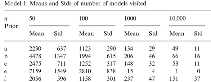
Table 3 records means and standard deviations of the number of visited models in the 50,000 recorded draws of the chain in model space (i.e., after the burn-in). Given that the model that generated the data is one of the 215"32,768 possible models examined, we would want this to be as small as possible. For
n"50 it is clear that the sample information is rather weak, allowing the chain to wander around and visit many models: as much as around a quarter of the total amount of models for prior g, and never less than 3.5% on average (prior i). The sampler visits fewer models asnincreases, and forn"1000 we already have very few visited models for prior g in particular and also for e. Of course, depending on the"eld of application, 1000 observations may well be considered quite a large sample. When 10,000 observations are available, that is enough to make the sampler stick to one model (the correct one) for priors e, g and h. Surprisingly, whereas prior h still leads to very erratic behaviour of the sampler with n"1000, it never fails to put all the mass on the correct model for the larger sample sizes. Even with 100,000 observations, priors d and f (though consistent) still make the sampler visit 240 and 110 models on average. For prior i this is as high as 287 models.
Table 4 indicates in what sense the di!erent Bayesian models tend to err if they assign posterior probability to alternative sampling models. In particular, Table 4 presents the means and standard deviations of the posterior probabilit-ies of including each of the regressors. As we know from (3.3), Model 1 contains regressors 1, 5, 7, 11 and 13 (indicated with arrows in Table 4). To save space, we shall only report these results forn"50 andn"1000, and we will not include prior c (for which results were virtually identical to prior a) and prior d. When
n"50, regressors z(1) and z(7) are almost always included. Since they are (almost) orthogonal to the other regressors, and their regression coe$cients are rather large in absolute value, this is not surprising. Regressor z
(11) is only correlated withz
Table 2
Model 1: Quartiles of ratio of posterior probabilities; true model versus best among the rest
n 50 100 500 1000 10,000
Prior
Q1 Q2 Q3 Q1 Q2 Q3 Q1 Q2 Q3 Q1 Q2 Q3 Q1 Q2 Q3
a 1.5 3.2 6.3 3.0 5.8 8.6 3.5 13.5 20.0 9.1 19.0 29.8 27.6 67.8 90.5
b 1.1 2.6 4.2 2.2 4.1 6.2 5.5 10.8 15.3 9.6 16.6 22.1 16.6 36.3 66.3
c 1.2 3.4 5.8 2.0 5.1 8.3 7.6 13.7 18.5 7.0 13.8 22.9 26.3 55.9 73.6
e 1.6 2.7 3.5 1.9 3.8 5.8 18.8 53.6 73.6 226.5 416.4 629.4 R R R
f 1.7 4.0 7.0 2.0 4.4 8.7 5.1 10.9 14.1 4.7 9.2 16.5 9.7 19.7 24.9
g 1.4 2.3 3.3 1.4 3.9 5.1 6.3 53.9 250.2 11.4 238.7 3625.8 R R R
h 1.2 2.3 2.8 1.9 2.8 3.9 2.9 4.9 5.7 5.9 10.6 12.9 R R R
i 1.1 4.3 9.8 2.1 6.5 12.5 4.3 8.8 12.8 4.8 8.4 13.0 6.0 10.9 14.6
C.
Ferna
&
ndez
et
al.
/
Journal
of
Econometrics
100
(2001)
381
}
Table 3
Model 1: Means and Stds of number of models visited
n 50 100 1000 10,000 100,000
Prior
Mean Std Mean Std Mean Std Mean Std Mean Std
a 2230 637 1123 290 134 29 49 11 20 5
b 4478 1347 1994 615 206 46 66 16 25 7
c 2475 711 1252 317 148 32 53 11 21 5
e 7159 1549 2810 838 15 4 1 0 1 0
f 2056 596 1158 301 237 47 151 37 110 24
g 8677 1608 3555 1204 3 1 1 0 1 0
h 5480 1353 3322 809 654 89 1 0 1 0
i 1176 451 758 222 288 51 288 55 287 53
coe$cients of opposite signs. The posterior probabilities of including regressors not contained in the correct model are all relatively small. Note that this is exactly where prior i excels, as the posterior probabilities of including incorrect regressors are much smaller than for the other priors. What is not clearly exempli"ed by Table 4 is that most priors tend to choose alternatives that are nested by Model 1 for small sample sizes, with the exception of priors d and h, which put considerable posterior mass on models that nest the correct sampling model. Table 4 informs us that forn"1000 the correct regressors are virtually always included. Only prior g has a tendency to choose models that are nested by Model 1. For the other priors there remain small probabilities of incorrectly including extra regressors (the smallest for prior e and the largest for priors d and h). Alternative models tend to nest the correct model for all priors, except prior g, with this and larger sample sizes.
5.2.2. Results under Model 2
Let us now brie#y present the results when the data are generated according to Model 2 in (3.4), the null model. Table 5 presents means and standard deviations of the posterior probability of the null model. It is clear that this is not an easy task (see also the discussion in Freedman, 1983; Raftery et al., 1997) and most priors lead to small probabilities of selecting the correct model. Overall, prior i does best for small sample sizes (followed by priors a and f), whereas larger sample sizes are most favourable to priors a and b. The behav-iour of prior i is quite striking: it appears that sample size has very little in#uence of the posterior probability of the correct model, making it a clear winner for values of n)100. Note that the other prior where g0
j does not depend on
Prior a b e f g h i Reg.
Mean Std Mean Std Mean Std Mean Std Mean Std Mean Std Mean Std
n"50
P1 0.98 0.07 0.98 0.07 0.97 0.09 0.98 0.07 0.96 0.09 0.98 0.06 0.98 0.10
2 0.22 0.17 0.29 0.14 0.33 0.10 0.21 0.17 0.35 0.09 0.36 0.13 0.13 0.13
3 0.25 0.18 0.31 0.14 0.35 0.11 0.24 0.18 0.37 0.10 0.38 0.13 0.15 0.12
4 0.27 0.19 0.33 0.15 0.37 0.11 0.25 0.19 0.39 0.10 0.40 0.13 0.21 0.21
P5 0.42 0.27 0.44 0.22 0.43 0.15 0.40 0.27 0.43 0.13 0.50 0.19 0.41 0.30
6 0.22 0.16 0.28 0.13 0.32 0.09 0.21 0.15 0.34 0.08 0.35 0.13 0.10 0.10
P7 0.94 0.14 0.94 0.13 0.90 0.15 0.94 0.15 0.87 0.15 0.94 0.12 0.86 0.22
8 0.22 0.16 0.29 0.14 0.32 0.10 0.21 0.15 0.34 0.08 0.36 0.13 0.13 0.14
9 0.21 0.14 0.28 0.12 0.32 0.08 0.20 0.14 0.34 0.07 0.35 0.11 0.12 0.11
10 0.21 0.14 0.28 0.12 0.32 0.08 0.20 0.13 0.34 0.07 0.35 0.11 0.11 0.08
P11 0.82 0.25 0.81 0.22 0.76 0.19 0.81 0.25 0.74 0.18 0.82 0.20 0.73 0.30
12 0.24 0.19 0.30 0.15 0.34 0.11 0.23 0.19 0.36 0.09 0.37 0.14 0.15 0.15
P13 0.39 0.27 0.43 0.23 0.44 0.18 0.38 0.27 0.45 0.15 0.49 0.20 0.33 0.28
14 0.27 0.22 0.32 0.19 0.36 0.13 0.25 0.22 0.37 0.11 0.39 0.16 0.15 0.16
15 0.22 0.15 0.28 0.12 0.33 0.08 0.21 0.15 0.35 0.07 0.36 0.11 0.15 0.16
n"1000
P1 1.00 0.00 1.00 0.00 1.00 0.00 1.00 0.00 1.00 0.00 1.00 0.00 1.00 0.00
2 0.07 0.11 0.09 0.12 0.00 0.01 0.11 0.13 0.00 0.00 0.16 0.10 0.11 0.07
3 0.06 0.08 0.08 0.08 0.00 0.01 0.09 0.09 0.00 0.00 0.15 0.07 0.11 0.08
4 0.05 0.06 0.07 0.07 0.00 0.01 0.08 0.08 0.00 0.00 0.14 0.06 0.10 0.07
P5 1.00 0.00 1.00 0.00 1.00 0.00 1.00 0.00 0.88 0.26 1.00 0.00 1.00 0.00
6 0.07 0.08 0.09 0.09 0.00 0.00 0.10 0.10 0.00 0.00 0.16 0.08 0.11 0.11
P7 1.00 0.00 1.00 0.00 1.00 0.00 1.00 0.00 1.00 0.00 1.00 0.00 1.00 0.00
8 0.06 0.07 0.08 0.08 0.00 0.00 0.10 0.10 0.00 0.00 0.15 0.08 0.10 0.06
9 0.06 0.06 0.08 0.08 0.00 0.00 0.10 0.09 0.00 0.00 0.15 0.07 0.11 0.09
10 0.06 0.07 0.08 0.08 0.00 0.00 0.10 0.09 0.00 0.00 0.15 0.07 0.12 0.13
P11 1.00 0.00 1.00 0.00 1.00 0.00 1.00 0.00 1.00 0.00 1.00 0.00 1.00 0.00
12 0.06 0.10 0.08 0.10 0.00 0.01 0.09 0.10 0.00 0.00 0.15 0.09 0.11 0.13
P13 1.00 0.00 1.00 0.00 1.00 0.00 1.00 0.00 0.78 0.34 1.00 0.00 1.00 0.00
14 0.05 0.04 0.07 0.05 0.00 0.00 0.08 0.06 0.00 0.00 0.14 0.05 0.13 0.14
15 0.06 0.07 0.07 0.08 0.00 0.00 0.09 0.09 0.00 0.00 0.14 0.07 0.11 0.07
C.
Ferna
&
ndez
et
al.
/
Journal
of
Econometrics
100
(2001)
381
}
Table 5
Model 2: Means and Stds of the posterior probability of the true model
n 50 100 500 1000 10,000 100,000
Prior
Mean Std Mean Std Mean Std Mean Std Mean Std Mean Std
a 0.0320 0.0269 0.0722 0.0494 0.2707 0.1338 0.3812 0.1543 0.7199 0.1346 0.8995 0.0529
b 0.0021 0.0028 0.0114 0.0124 0.1394 0.1055 0.2606 0.1506 0.6910 0.1441 0.8960 0.0568
c 0.0099 0.0081 0.0238 0.0157 0.0994 0.0505 0.1494 0.0715 0.4148 0.1201 0.7080 0.1009
e 0.0003 0.0003 0.0006 0.0006 0.0034 0.0036 0.0066 0.0066 0.0427 0.0300 0.1570 0.0938
f 0.0407 0.0322 0.0764 0.0492 0.1787 0.0959 0.2216 0.1050 0.3569 0.1220 0.4733 0.1235
g 0.0001 0.0002 0.0002 0.0002 0.0005 0.0005 0.0005 0.0006 0.0009 0.0008 0.0014 0.0015
h 0.0010 0.0012 0.0011 0.0012 0.0016 0.0015 0.0014 0.0014 0.0013 0.0011 0.0014 0.0014
i 0.1599 0.0862 0.1658 0.0842 0.1833 0.0870 0.1790 0.0891 0.1780 0.0886 0.1862 0.0815
Ferna
&
ndez
et
al.
/
Journal
of
Econometrics
100
(2001)
381
}
427
Table 6
Model 2: Quartiles of ratio of posterior probabilities; true model versus best among the rest
n 50 100 1000 10,000 100,000
Prior
Q1 Q2 Q3 Q1 Q2 Q3 Q1 Q2 Q3 Q1 Q2 Q3 Q1 Q2 Q3
a 2.4 4.4 7.0 3.1 6.2 9.2 6.0 16.1 24.8 30.0 60.0 86.2 78.7 202.4 272.1
b 2.1 5.2 7.0 3.7 6.7 9.7 7.4 22.1 28.9 18.4 45.7 79.6 64.1 153.8 253.2
c 1.3 1.8 2.1 1.2 2.2 2.7 2.0 4.1 7.1 6.3 15.2 21.8 16.1 40.3 70.2
e 1.1 2.1 2.8 1.2 2.5 3.2 2.2 3.9 5.2 3.1 6.6 9.4 6.1 11.2 16.7
f 2.4 5.3 7.5 3.5 6.8 9.3 4.9 11.4 17.5 8.1 15.7 25.3 12.9 26.9 36.2
g 0.5 1.5 2.6 0.6 1.6 2.6 0.9 2.3 3.2 1.3 2.6 3.5 1.8 3.4 4.2
h 1.2 2.3 3.2 1.3 2.5 3.2 1.3 2.7 3.2 1.7 2.7 3.5 1.6 2.5 3.1
i 4.2 8.2 13.4 5.5 10.7 13.7 4.6 9.8 14.3 6.3 10.6 14.1 4.3 9.2 14.4
C.
Ferna
&
ndez
et
al.
/
Journal
of
Econometrics
100
(2001)
381
}
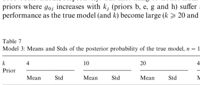
Table 7
Model 3: Means and Stds of the posterior probability of the true model,n"100
k 4 10 20 40
Prior
Mean Std Mean Std Mean Std Mean Std
a 0.6993 0.1616 0.4016 0.1263 0.1745 0.0772 0.0111 0.0113
b 0.6562 0.1570 0.5970 0.1908 0.0007 0.0020 0.0000 0.0000
c 0.6408 0.1648 0.3034 0.1042 0.1116 0.0516 0.0097 0.0086
d 0.4599 0.1301 0.1589 0.0430 0.0115 0.0048 0.0000 0.0000
e 0.7269 0.1210 0.1947 0.1103 0.0000 0.0001 0.0000 0.0000
f 0.6971 0.1618 0.3986 0.1256 0.1722 0.0761 0.0107 0.0107
g 0.8036 0.1059 0.0604 0.0439 0.0000 0.0000 0.0000 0.0000
h 0.5503 0.1274 0.1676 0.0421 0.0035 0.0015 0.0000 0.0000
i 0.5084 0.1442 0.4015 0.1262 0.3145 0.1352 0.0949 0.1074
the ratio of the posterior probabilities of Model 2 and the best other model are presented. Only prior g forn)1000 leads to a"rst quartile below unity. Clearly, prior i does best forn)100 and prior a does best for largern. The di$culty of pinning down the correct (null) model can also be inferred from the number of visited models (not presented in detail). Some priors (like d, e, g and h) make the chain wander a lot for small sample sizes. Priors g and h retain this problematic behaviour even for sample sizes as large as 100,000. Interestingly, whereas prior g leads to (very slow) improvements asnincreases, the bad behaviour with prior h seems entirely una!ected by sample size, as remarked above. Of course, we know from the theory in the appendix that priors h and i do not lead to consistent Bayes factors in this case. Whereas prior h visits on average about 12,500 models for any sample size, prior i visits around one tenth of that. The number of models visited is relatively small for priors i and a, which seem to emerge as the clear winners from the posterior results under Model 2, respective-ly, for small and large values ofn.
5.2.3. Results under Model 3
Now the setup of the experiment is slightly di!erent, as we contrast various model sizes (in terms ofk) and only two sample sizes. We would expect that the task of identifying the true model becomes harder askincreases, since the total number of models inMincreases dramatically from 16 (fork"4) to 1.1]1012 (fork"40). Of course, this may be partly o!set by the fact thatpremains the same, so that the theoretical coe$cient of determination grows withk. Tables 7 and 8 present the posterior probability of Model 3 in (3.5) withn"100 and 1000 observations, respectively. The"rst thing to notice from Table 7 is that priors whereg
0j increases with kj (priors b, e, g and h) su!er a large drop in
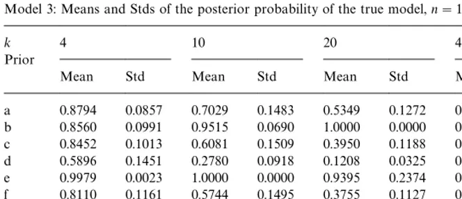
Table 8
Model 3: Means and Stds of the posterior probability of the true model,n"1000
k 4 10 20 40
Prior
Mean Std Mean Std Mean Std Mean Std
a 0.8794 0.0857 0.7029 0.1483 0.5349 0.1272 0.2366 0.1699
b 0.8560 0.0991 0.9515 0.0690 1.0000 0.0000 0.6499 0.4769
c 0.8452 0.1013 0.6081 0.1509 0.3950 0.1188 0.1853 0.0788
d 0.5896 0.1451 0.2780 0.0918 0.1208 0.0325 0.0459 0.0054
e 0.9979 0.0023 1.0000 0.0000 0.9395 0.2374 0.0000 0.0000
f 0.8110 0.1161 0.5744 0.1495 0.3755 0.1127 0.1972 0.0685
g 1.0000 0.0000 1.0000 0.0001 0.0015 0.0036 0.0000 0.0000
h 0.9958 0.0035 0.9357 0.0164 0.1731 0.1957 0.0222 0.0070
i 0.5150 0.1349 0.4174 0.1305 0.4030 0.1172 0.3170 0.1856
prior g). Interestingly, prior i, which is decreasing inkdoes not su!er from this, and performs quite well forn"100. In fact, priors a, f and i all do remarkably well in identifying the true model from a very large model space on the basis of a mere 100 observations. The results fork"40 appear less convincing, but we have to bear in mind that the posterior probability of the correct model multiplies the corresponding prior probability by more than 1]1010with these priors.
When we consider Table 8, corresponding to n"1000, we note that most priors bene"t from the larger sample size. Only prior i leads to virtually the same posterior probabilities as with the smaller sample (except for large k). In line with the larger sample sizen, the drop in posterior probability for the priors with
g
0j increasing inkj now tends to occur at a higher value ofkthan in Table 7.
5.3. Predictive inference
5.3.1. Results under Model 1
As discussed in Section 4.3 we shall condition our predictions on values of the regressorsz
f. In all, we chooseq"19 di!erent vectors for these regressors, and
we shall focus especially on those vectors that lead to the minimum, median and maximum value for the mean of the sampling model. We shall denote these regressors asz
.*/, z.%$andz.!9, respectively. In our particular case,z.*/ will be
more extreme thanz
.!9 for Model 1. For Model 3, both are roughly equally
extreme.
Firstly, Table 9 presents the median of¸PS(z
f, y, Z) in (3.8), computed across
Table 9
Model 1: conditional medians of¸PS(z f,y,Z)
n 50 100 1000 10,000 100,000
z
.*/ z.%$ z.!9 z.*/ z.%$ z.!9 z.*/ z.%$ z.!9 z.*/ z.%$ z.!9 z.*/ z.%$ z.!9
a 2.471 2.425 2.428 2.391 2.389 2.391 2.334 2.355 2.348 2.330 2.352 2.347 2.331 2.350 2.345
b 2.480 2.422 2.431 2.409 2.390 2.385 2.334 2.355 2.347 2.330 2.352 2.347 2.331 2.350 2.345
c 2.471 2.424 2.433 2.397 2.389 2.389 2.334 2.355 2.347 2.330 2.352 2.347 2.331 2.350 2.345
e 2.691 2.448 2.475 2.507 2.406 2.410 2.358 2.356 2.354 2.332 2.351 2.347 2.332 2.351 2.345
f 2.474 2.428 2.428 2.393 2.389 2.391 2.333 2.355 2.347 2.329 2.352 2.346 2.331 2.350 2.345
g 2.836 2.470 2.530 2.636 2.423 2.463 2.475 2.378 2.412 2.444 2.371 2.391 2.417 2.362 2.379
h 2.492 2.430 2.440 2.450 2.392 2.395 2.418 2.362 2.381 2.423 2.367 2.382 2.422 2.364 2.382
i 2.488 2.421 2.428 2.392 2.389 2.392 2.333 2.355 2.347 2.329 2.352 2.346 2.332 2.350 2.345
Ferna
&
ndez
et
al.
/
Journal
of
Econometrics
100
(2001)
381
}
427
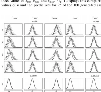
Fig. 1. Model 1: Predictive densities,n"50, 100, 1000 and 10,000.
in Section 4.3. Of course,¸PSin (3.8) is only a Monte Carlo approximation to this integral (based on a mere 100 draws), so this lower bound is not always strictly adhered to. The Monte Carlo (numerical) standard error corresponding to the numbers in Table 9 is roughly equal to 0.02 forn"50, decreases to about 0.01 for n"100 and then quickly settles down at about 0.007 as n becomes larger. Under priors a, b, c, f and i we are predicting the sampling density virtually exactly with samples of sizen"1000 or more. These same priors also lead to the best results for smallern. Prior e performs worse for small samples, while priors g and h tend to be even further from the actual sampling density and do not lead to perfect prediction even with 100,000 observations.
In order to"nd out more about the di!erences between the predictive density in (3.6) and the sampling density in (3.3), we can overplot both densities for the three values ofz
.*/,z.%$ andz.!9. Fig. 1 displays this comparison for di!erent
cluttering the graphs). The drawn line corresponds to the actual sampling density. Since the predictives from priors a}c, f and i are very close for all sample sizes, we shall only present the graphs for priors a, e, g and h. It is clear that for
n"50 substantial uncertainty remains about the predictive distribution: di!er-ent samples can lead to rather di!erdi!er-ent predictives. They are, however fairly well calibrated in that they tend to lie on both sides of the actual sampling density for priors a}c, f and i and there is no clear tendency towards a di!erent degree of concentration. These are exactly the priors for whichg
0j takes on fairly small
values (for prior ig
0j"0.0044 and for the others it is in between 0.02 and 0.08).
Priors e, g and h lead to much larger values forg
0j(in the range 0.16 to 0.41) and
show a clear tendency for the predictive densities to be somewhat biased towards the median when conditioning on z
.*/ and z.!9. In addition, these
priors induce predictives that are, on average, less concentrated than the sampling density, even for very large sample sizes. This behaviour can easily be understood once we realize that the location of (3.6) (the posterior mean of a#z@
f,jbj) is clearly shrunk more towards the sample meany asg0j becomes
larger. This is, of course, in accordance with the zero prior mean forb
jand the g-prior structure in (2.15). In addition, predictive precision decreases withg
0j,
which explains the systematic excess spread of the predictives with respect to the sampling density for priors e, g and h. As sample size increases, the predictive distributions get closer and closer to the actual sampling distribution, and for
n"1000 or larger the e!ect of shrinkage due tog
0j has become negligible for
prior e (g
0j is then equal to 0.07 forkj"5) whereas it persists for priors g and
h even with 100,000 observations (where g
0j takes the value 0.14 and 0.16,
respectively). The graph for the latter case is not presented in Fig. 1, but it is very close to that withn"10,000.
We can also compare overall predictive performance, through considering ¸PS(z
f,y,Z) for the 19 di!erent values ofzfand the 100 samples of (y,Z). This
leads to the results presented in Table 10, where the medians (computed across the 1900 sample-z
f combinations) are recorded for the di!erent priors and
sample sizes. Monte Carlo standard errors corresponding to the entries in Table 10 are approximately 0.005 forn"50, about 0.0025 forn"100 and decrease to around 0.0015 for largern. Clearly, whereas all priors except for priors e and g lead to comparable predictive behaviour for very smalln, the fact thatg
0j is
large and constant inn makes prior h lose ground with respect to the other priors asnincreases. Prior g always performs worse than priors a through f and prior i. Note that the latter priors lead to median LPS values that are roughly equal to the theoretical minimum of 2.335, implying perfectly accurate predic-tion, forn*10,000 (which may, of course, be quite a large sample size for some applications). Priors a}c, f and i perform best overall, and are already quite close to perfect prediction forn"1000.
Table 10
Model 1: medians of¸PS(z
f,y,Z)
n 50 100 1000 10,000 100,000
a 2.427 2.382 2.339 2.334 2.333
b 2.427 2.383 2.339 2.334 2.333
c 2.424 2.381 2.339 2.334 2.333
e 2.473 2.416 2.347 2.336 2.334
f 2.428 2.382 2.339 2.334 2.333
g 2.502 2.452 2.393 2.374 2.363
h 2.433 2.452 2.369 2.367 2.366
i 2.428 2.382 2.339 2.334 2.334
to the 1, 5, 25, 50, 75, 95, and 99 sampling percentile. The quartiles of these numbers, calculated over all 1900 sample-z
fcombinations, con"rm that priors
a}c, f and i lead to better predictions for small sample sizes, where the predictives from e, g and h are too spread out. Starting atn"1000, prior e predicts well, whereas the inaccurate predictions with priors g and h persist even for very large sample sizes. For space considerations, these results are not presented here, but are obtainable upon request from the authors. In addition, Fig. 1 shows that most of the spread in the percentiles for priors g and h withn*10,000 is due to the bias towards the median (shrinkage).
5.3.2. Results under Model 2
As mentioned in Section 5.2.2, it is hard to correctly identify the null model when we generate the data from such a model. On the other hand, prediction seems much easier than model choice. This can immediately be deduced from predictive percentiles (not reported, but obtainable upon request). The incor-rectly chosen models are such that they do not lead our predictions (averaged over all the chosen models as in (3.6)) far astray. Even with just 50 observations median predictions are virtually exact, and the spread around these values is relatively small. Moreover, this behaviour is encountered for all priors. When sample size is up to 1000, prediction is near perfect for all priors. For this model the issue of shrinkage is, of course, less problematic.
5.3.3. Results under Model 3
Table 11 presents the medians of the conditional ¸PS(z
f,y,Z) as in (3.8),
computed with v"100 out-of-sample observations. The theoretical minimum corresponding to perfect prediction is 2.112, and Monte Carlo standard errors for the numbers in Table 11 are of the order 0.008 fork"4 and vary from 0.01 to 0.04 for k"40. The most obvious "nding from Table 11 is the poor performance of priors e, g and h, which correspond to the largest values ofg
0j.
Table 11
Model 3: conditional medians of¸PS(z
f,y,Z),n"100
k 4 10 20 40
z
.*/ z.%$ z.!9 z.*/ z.%$ z.!9 z.*/ z.%$ z.!9 z.*/ z.%$ z.!9
a 2.151 2.110 2.138 2.154 2.139 2.168 2.220 2.218 2.224 2.555 2.453 2.490 b 2.153 2.111 2.133 2.200 2.164 2.202 2.646 2.529 2.588 3.365 3.161 3.226 c 2.153 2.111 2.136 2.160 2.142 2.168 2.227 2.223 2.230 2.574 2.467 2.492 d 2.173 2.113 2.151 2.244 2.195 2.287 2.592 2.502 2.562 3.215 3.076 3.120 e 2.192 2.120 2.171 2.449 2.293 2.584 3.089 2.802 3.003 3.802 3.422 3.764 f 2.151 2.110 2.138 2.154 2.140 2.168 2.221 2.218 2.224 2.557 2.461 2.497 g 2.240 2.129 2.221 2.615 2.395 2.883 3.328 2.916 3.237 4.034 3.552 4.024 h 2.193 2.119 2.169 2.341 2.248 2.434 2.832 2.648 2.769 3.434 3.251 3.409 i 2.155 2.113 2.133 2.154 2.139 2.168 2.212 2.219 2.232 2.472 2.401 2.471
an increasing function ofk
j. The best forecasting performance is observed for
priors a, c, f and i, which all do a very good job, even in the context of a very large model set.
5.4. Recommendations
On the basis of the posterior and predictive results mentioned above, we can o!er the following advice to practitioners, although we stress that it is probably impossible to recommend a choice for g
0j that performs optimally in all
situations. Nevertheless, it appears that a strategy using prior i for the smallest values ofn, in particular wheren)k2, and prior a for those cases wheren'k2 would do very well in most situations. It would actually lead to the best or close to the best results in all comparisons made above. The only substantial improve-ment to that strategy would be to choose prior e instead of prior a for Model 1. Whereas prediction would be slightly less good, posterior probabilities of the true model would be quite a bit higher. A similar, but less clear-cut, trade-o!can be observed for Model 3. However, this strategy appears more risky, as it would lead to a dramatic fall in performance for Model 2 on the same criterion (see Table 5). Of course, Model 2 might be considered a very unusual situation, so that some practitioners may well adopt this more risky strategy, especially if they are more interested in posterior results, rather than in predicting. As a general recommendation, however, we would propose the&safe'strategy.
Note that the latter implies choosing the prior rule with the smallest value of
g0
j, i.e., it amounts to
g 0j"
1
and is quite unlikely to lead us far astray, sinceg
0jwill never take large values in
situations of practical relevance. This prior will combine the consistency proper-ties of prior a with the impressive small sample performance of prior i.
6. An empirical example: Crime data
The literature on the economics of crime has been critically in#uenced by the seminal work of Becker (1968) and the empirical analysis of Ehrlich (1973, 1975). The underlying idea is that criminal activities are the outcome of some rational economic decision process, and, as a result, the probability of punishment should act as a deterrent. Raftery et al. (1997) have used the Ehrlich data set corrected by Vandaele (1978). These are aggregate data for 47 U.S. states in 1960, which will be used here as well.
The single-equation cross-section model used here is not meant to be a serious attempt at an empirical study of these phenomena. For example, the model does not address the important issues of simultaneity and unobserved heterogeneity, as stressed in Cornwell and Trumbull (1994), and the data are at state level, rather than individual level, but we shall use it mainly for comparison with the results in Raftery et al. (1997), who also treat it as merely an illustrative example. We shall, thus, consider a linear regression model as in (1.1), where the dependent variable, y, groups observations on the crime rate, and the 15 regressors in Z are given by: percentage of males aged 14}24, dummy for southern state, mean years of schooling, police expenditure in 1960, police expenditure in 1959, labour force participation rate, number of males per 1000 females, state population, number of nonwhites per 1000 people, unemployment rate of urban males aged 14}24, unemployment rate of urban males aged 25}39, wealth, income inequality, probability of imprisonment, and average time served in state prisons. All variables except for the southern dummy are transformed to logarithms.
Table 12
Crime data: models with more than 2% posterior probability Prob. (%) Included regressors
1 3.61 1 3 4 11 13 14
2 3.48 1 3 4 9 11 13 14
3 2.33 1 3 5 11 13 14
4 2.31 1 3 4 11 13
5 2.29 1 3 4 13 14
6 2.20 1 3 5 9 11 13 14
7 2.05 3 4 8 9 13 14
8 2.02 1 3 4 9 13 14
Raftery et al. (1997, Table 3), we estimate the total model probability covered by the chain to be 99.3%, thus corroborating our earlier conclusion of convergence. Note that this run takes a mere 34 seconds on a 200 MHz PPC603ev-based Macintosh 3400c laptop computer.
Table 12 presents the 8 models that receive over 2% posterior probability. Seven of these models are among the ten best models of Raftery et al. (1997). In general, model probabilities are roughly similar, even though our prior is quite di!erent from the one proposed in Raftery et al. (1997). In particular, we only require the user to choose the functiong
0j, and choosing it in accordance with
our"ndings in Section 4 leads to results that are reasonably close to those with the rather laboriously elicited prior of Raftery et al. (1997). The second best model in Table 12 is the one that is chosen by the Efroymson stepwise regression method, as explained in Raftery et al. (1997), and is the model with highest posterior probability in the latter paper. If we use prior a in our framework, we also get this as the model with highest posterior probability. Generally, prior a leads to a more di!use posterior model probability and larger models.