Estimation of evapotranspiration from a field
of linseed in central Italy
R. Casa
a,∗, G. Russell
b, B. Lo Cascio
aaDipartimento di Produzione Vegetale, Università degli Studi della Tuscia, Via S. Camillo de Lellis, 01100 Viterbo, Italy bInstitute of Ecology and Resource Management, The University of Edinburgh, West Mains Road, Edinburgh EH9 3JG, Scotland, UK
Received 6 December 1999; received in revised form 14 June 2000; accepted 14 June 2000
Abstract
A study was carried out in central Italy into the evapotranspiration from linseed (Linum usitatissimum L.). In particular, the objectives were to (a) evaluate the accuracy of daily evapotranspiration estimates from partially incomplete Bowen ratio data; (b) measure seasonal evapotranspiration from linseed; (c) test the FAO 56 method for estimating crop coefficients for linseed and (d) calculate the surface resistance of the crop as a function of soil water status. The study was carried out on a crop of linseed growing in a 1.1 ha field near Viterbo using Bowen ratio apparatus. Soil water content and green area index were also monitored. It was found that (1) daily evapotranspiration could be estimated from partially incomplete Bowen ratio data on a continuous basis throughout the growing season; (2) the linseed crop lost 240 mm over the 100-day growing season; (3) measured crop coefficients agreed with those obtained using the FAO 56 methodology; (4) surface resistance could be expressed as a function of green area index and soil water deficit seemed to have an indirect effect by hastening leaf senescence. © 2000 Published by Elsevier Science B.V.
Keywords: Bowen ratio; Evapotranspiration; Linseed; Linum usitatissimum L.; Penman–Monteith equation; Water use
1. Introduction
In recent decades, many complex models have been proposed for the analysis and prediction of crop wa-ter use. However, simplicity is essential for practical application at the farm or field level, so complicated mechanisms and processes are often reduced to em-pirical coefficients. The procedure most widely used by agronomists for the estimation of crop water re-quirements has probably been the FAO 24 approach (Doorenbos and Pruitt, 1977), where the evapotranspi-ration from a well-watered crop is estimated by
multi-∗Corresponding author. Tel.:+390-761-357-554; fax:+390-761-357-558.
E-mail address: [email protected] (R. Casa).
plying the evaporation from a reference crop by a crop coefficient Kc that takes into account the differences in albedo, emissivity, soil heat flux, aerodynamic and surface resistances between the crop considered and the reference crop. These depend to a large extent on the leaf area index of the crop and its height and thus on the phenological stage. It has been shown that Kc is site-specific (Hanks, 1985) with the main sources of variation being the frequency of wetting of the soil (Jagtap and Jones, 1989) and the degree of coupling between the vapour pressure deficit at the canopy sur-face and in the free airstream (Jarvis and McNaughton, 1986). Variation also arises from the differences in canopy development between locations. Less variable results are obtained when evaporation from the soil is considered separately and Kcis partitioned into a basal 0168-1923/00/$ – see front matter © 2000 Published by Elsevier Science B.V.
crop and a soil coefficient (Wright, 1982). The coeffi-cients can then be used more safely in locations other than those in which they were originally determined (Ritchie and Johnson, 1990). The actual values of Kc obviously depend on the method used to compute reference evapotranspiration and the lack of agree-ment between the various models (Choisnel et al., 1992) prevents the creation of a unique set of Kc values (Howell et al., 1995).
The FAO 24 methodology has recently been re-vised (Allen et al., 1998). This methodology will be referred to, in the present paper, as FAO 56. The ref-erence crop evapotranspiration (E0), now defined for a ‘hypothetical crop’ resembling grass (Allen et al., 1994), is to be computed using the Penman–Monteith equation (Monteith, 1965). In addition, an extended procedure for adjusting E0 to actual crops has been developed (Allen et al., 1996). This procedure takes into account evaporation from the soil surface, and sub-optimal growth conditions such as water stress and salinity, which result in a reduced leaf area index or an increased surface resistance. A water balance model of the surface soil layer based on the two-stage drying model described by Ritchie (1972) is used to estimate soil evaporation and a water balance model of the root zone is added when soil water availability is sub-optimal.
Independent tests of the FAO 56 procedure are now needed in order to test its validity for a wide range of crop species and environments. Lysimeters have of-ten been used to provide the ‘true’ evapotranspiration (Wright, 1982; Pruitt, 1991). However, some authors have claimed that measurement errors are more com-mon than usually thought (Allen et al., 1994). Increas-ingly, the Bowen ratio method is employed to estimate crop evapotranspiration and calculate crop coefficients (Hsiao et al., 1985; Grattan et al., 1998) because of its portability and relative cheapness compared with the other micrometeorological techniques. Errors in the Bowen ratio estimate of evapotranspiration are com-monly considered to be of the order of 10% (Sinclair et al., 1975; Angus and Watts, 1984). However, recent improvements in the instrumentation and careful data analysis should enable this error to be reduced (Malek and Bingham, 1993; Allen et al., 1994). The removal of erroneous data (Tattari et al., 1995) can result in substantial gaps in the record which can be filled us-ing procedures that have been proposed for estimation
of evapotranspiration by remote sensing (Sugita and Brutsaert, 1991; Zhang and Lemeur, 1995).
In the present paper, evapotranspiration of lin-seed (Linum usitatissimum L.) was estimated using the Bowen ratio technique during a growing season in central Italy. Linseed, grown for the production of industrial oil, and its close relative, flax has a world-wide cultivation area from Canada to India representing a wide range of environmental and man-agement conditions. The Kc values reported in FAO 56 and FAO 24 procedures come from a limited num-ber of experiments carried out in Arizona and eastern Europe and require to be validated for Mediterranean conditions. Data on the effect of soil water status on the actual water use of linseed in field conditions are also lacking and this hinders the development and ap-plication of decision support systems for conditions where shortage of water is important (Casa et al., 1997). Most of the relevant informations come from experiments carried out in India (Gupta and Agrawal, 1977; Tiwari et al., 1988; Dutta et al., 1995) where conditions are different from that in Italy.
The objectives of the present study were thus the following.
1. To evaluate the accuracy of daily evapotranspi-ration estimates from partially incomplete but quality-checked Bowen ratio data.
2. To estimate linseed water use using the Bowen ratio method.
3. To test the FAO 56 methodology for estimating Kc. 4. To investigate the effect of water shortage on evap-otranspiration by calculating the surface resistance of the crop.
2. Methods
2.1. Site description and sampling procedures
and Scharafat (1964) observed linseed roots reaching a depth of 1.20 m in Germany and Gupta and Agrawal (1977) showed that linseed can take up soil water from a depth of 1.0 m so the complete soil profile was ac-cessible to the roots. There was no water table within the reach of the roots. Phosphorus and potassium fer-tilizers were applied during seedbed preparation using 69 kg P2O5ha−1 and 75 kg K2O ha−1. Nitrogen, to-talling 92 kg ha−1, was applied as urea, half at sowing and half at the ‘buds visible’ stage of development. Emergence was complete by 24 March, at which time the plant population density was 550 plants m−2. Samples of above-ground plant material for growth analysis and leaf area determination were harvested weekly throughout the growing period using three replicate 0.5 m2quadrats. Green area index (GAI) was defined as the area of one side of the green leaf blades per unit area of land surface (Casa et al., 1999). The area of the green stems was ignored as calculations showed that it could be neglected without introducing significant errors. GAI is a more appropriate mea-sure of the transpiring area of the crop than leaf area index when the foliage is senescent. The crop was combine-harvested at maturity on 10 July, when it had lost all green colour.
Soil water content was measured weekly for four layers (0.00–0.10, 0.10–0.20, 0.20–0.40 and 0.40–0.60 m) at four locations in the field using the gravimetric method. Soil moisture was converted to a volumetric basis using bulk densities measured in the field at the end of the growing season for the same locations and layers as the gravimetric samples, using the excavation method of Blake and Hartge (1986). Pressure plate measurements of field capacity (−0.03 MPa) and wilting point (−1.5 MPa) were used to compute the profile available soil water. The soil water deficit (SWD), i.e. the amount of water needed to restore the profile to field capacity, was estimated by adding daily evapotranspiration (calculated using the Bowen ratio method) to, and subtracting rainfall from, the SWD of the previous day, subject to the usual constraint that the SWD cannot be negative. The calculation was started on the 1 April, 17 days after sowing (DAS), when the SWD could be accu-rately derived from soil moisture measurements. An independent estimate of SWD in the upper 0.60 m obtained from the measurements of soil moisture was used to check the validity of the computed values.
The fraction of solar radiation intercepted was measured throughout the growing season using tube solarimeters (Delta-T Devices, Cambridge, England). One solarimeter was positioned above the canopy and six below at randomly chosen locations in the field. The solarimeters were orientated at right angles to the rows, which were aligned approximately north-south. The fraction of the ground covered by the vegetation was estimated from the fractional radiation intercep-tion using the relaintercep-tionship of Steven et al. (1986) for barley, which has a similar leaf angle distribution.
2.2. Bowen ratio measurements and data processing
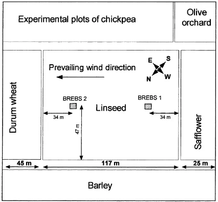
Two Bowen ratio energy balance systems (BREBS, Campbell Scientific) were installed in the field 34 m from the NE (BREBS2) and SW (BREBS1) edges and 47 m from the other two sides (Fig. 1). As the pre-vailing wind during the growing season was from the south-west, the fetch from the two units was normally either 34 (BREBS1) or 83 m (BREBS2). The net radiometers were moved upwards periodically to keep them about 1.0 m above the vegetation surface. Tem-perature and vapour pressure gradients above the crop were measured using two unshielded, unaspirated 76mm chromel–constantan thermocouples and one precision-cooled mirror dewpoint hygrometer (model Dew 10, General Eastern Corp., USA) for each
system. The lower arm was raised during the growing season to keep it 0.30 m above the vegetation surface while the distance between arms was kept constant at 0.60 m. For each BREBS, two soil heat flux plates were buried at a depth of 80 mm in the soil and four spatial-average, 40 gauge, chromel–constantan ther-mocouples were buried at depths of 20 and 60 mm. The soil heat flux at the surface (G) was computed by adding the average heat fluxes sensed by the plates to the energy stored in the soil layer above them. The storage term was calculated by multiplying the rate of change in soil temperature over the 20 min averaging period by the soil heat capacity (Malek, 1993) esti-mated from the interpolated volumetric soil moisture content of the 0.00–0.10 m soil layer.
Latent and sensible heat fluxes, which were av-eraged over 60 min periods, were computed by the equations usually employed in this method (see e.g. Malek and Bingham, 1993). The temperature and vapour pressure gradients for the whole dataset were carefully examined for systematic errors caused by contamination of the thermocouples. Data from the two BREBS were averaged if both were available, otherwise data from the functioning system were used. Erroneous data were rejected using an algo-rithm with the criteria specified by Ohmura (1982) which takes into account the resolution limits of the thermometers and hygrometers (±0.006◦C and ±0.01 kPa, respectively in this case). Following Heilman and Brittin (1989), data were also discarded for periods when the fetch, as calculated from wind direction, was less than twenty times the height of the arms. Stannard (1997) confirmed theoretically that the Bowen ratio method requires less fetch than the eddy covariance method.
Daytime latent heat flux was estimated from the remaining data assuming a constant evaporative frac-tion (Sugita and Brutsaert, 1991). Although Zhang and Lemeur (1995) showed that the evaporative fraction tended to be higher in the morning or evening and that it was more variable on cloudy days, most of the evapotranspiration from a crop takes place in the cen-tral part of clear days when the evaporative fraction tends to be most stable. The evaporative fraction was calculated as
where the subscript i refers to the ith measurement; n is the total number of available daytime measure-ments; E and H refer to latent and sensible heat fluxes, respectively.
The daytime latent heat flux was calculated as
Ed=feQd (2)
where Qd is the available energy:
Qd= Z t2
t1
(Rn−G)dt (3)
in which Rn is the net radiation, G the soil heat flux and the integration period (t2−t1) that part of the day when Rnwas positive, i.e. approximately the hours of daylight. The daytime latent heat flux was then con-verted into daily actual evapotranspiration (Ea) in mm per day assuming that night-time evapotranspiration could be neglected.
To assess the validity of this approach when data were missing, tests were carried out by removing in-creasing amounts of data for three days when all mea-surements were available, and comparing the estimates of evapotranspiration with those obtained using all the data. This test was done using fluxes averaged over 20 min to maximise the amount of data used. Day 78 after sowing (DAS), i.e. the 1 June, was charac-terised by completely clear skies, day 71 (25 May) was predominantly clear and day 86 (9 June) was largely cloudy. From 5 to 60% of the data (in 5% increments) was deleted at random for each of the days. The re-sultant 12 tests were repeated 10 times for each day using a different set of random numbers. It was ex-pected that the accuracy of the estimates of Eawould decline as fewer measurements were available, partic-ularly, when the missing data were from the central part of the day.
2.3. Reference evapotranspiration, crop coefficients and surface resistance
pressure which was computed from Bowen ratio dew-point temperature measurements. Although the actual vapour pressure was not measured in standard conditions, the data were considered to be more reli-able than those derived from the hair hygrometer at the agro-meteorological station.
The ‘measured’ crop coefficient (Kc) was calculated as (Ea/E0) and compared with the estimates obtained using the FAO 56 methodology (Allen et al., 1998) in which the estimated crop coefficient Kceis partitioned into a baseline crop coefficient (Kcb) defined as the ratio of crop to reference evapotranspiration when the soil surface is dry and transpiration is occurring at the potential rate and a coefficient accounting for surface soil evaporation (Ke). To take account of water stress, Kcbis multiplied by a coefficient Kswhich is equal to 1.00 till half the available water is used up and which then declines linearly to zero when all the available water in the rooting zone has been used up:
Ea=(KcbKs+Ke)Eo (4)
The term in brackets in Eq. (4) is called Kc adj. Fol-lowing the procedures in FAO 56, Kcbwas calculated from the measured crop growth stage and plant height and corrected to take account of the maximum ground cover. Keand Kswere estimated daily.
Following Russell (1980), daily values of linseed surface (canopy) resistance were computed by inver-sion of the Penman–Monteith equation using inte-grated daily net radiation, soil heat flux and mean vapour pressure deficit measured in the linseed field, windspeed and temperature from the meteorological station and estimated Ea. Aerodynamic resistance was computed using the equation recommended by FAO (Allen et al., 1998), without a stability correction.
3. Results
3.1. Evaluation of the errors in the evapotranspiration estimates
After rejection of clearly erroneous Bowen ratio data, 44% (BREBS 1) and 82% (BREBS 2) of the data remained and on many occasions estimates were avail-able from both the systems. BREBS 1 had more data failures due to water vapour condensing in the plastic tubing. Although 40% of the pairs of observations
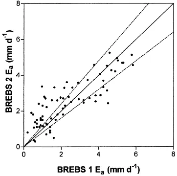
dif-Fig. 2. Comparison of daily actual evapotranspiration (Ea)
esti-mated from two different Bowen ratio energy balance systems (BREBS). Dashed lines represent±20% of the 1:1 Eavalues.
fered by no more than 0.5 mm per day (Fig. 2), the ratio of BREBS 1 to BREBS 2 estimates was less than one for low rates of evapotranspiration rates and greater than one at high rates and only 31% of the data fell within±20% of the 1:1 line (Fig. 2). The discrepancy between the two systems was partly attributed to their positions in the field which resulted in different fetch conditions (Fig. 1). However, the rate of evapotranspi-ration was not strongly correlated with wind direction and the effect of fetch was not consistent enough to reject one or other of the observations. When there were two estimates, an average was therefore taken.
The assumption that night-time evapotranspiration was negligible, was tested for the same three days. By considering only daytime evapotranspiration, underes-timates of 24 h Eaby 1, 2 and 6% were introduced for days 71, 78 and 86, respectively. The result for day 86 can be explained by the higher night-time windspeed (reaching a maximum of 2.5 m s−1) compared to other two days in which there was virtually no wind (max-ima less than 0.5 m s−1). However, the absolute error was similar (less than 0.1 mm per day) for the three days.
3.2. Water use by the linseed crop
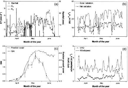
Fig. 4 shows the seasonal progression of actual evapotranspiration (Ea) of the linseed crop throughout the growing season as well as the trend of the main meteorological and crop factors that influenced Ea. As expected, Earates fell below reference
evapotranspira-Fig. 4. Seasonal trends of (a) reference (E0), actual evapotranspiration (Ea) and rainfall; (b) solar radiation and net radiation measured
over linseed; (c) fractional ground cover and green area index (GAI) and (d) windspeed and vapour pressure deficit.
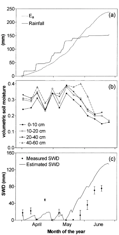
Fig. 5. (a) Cumulative rainfall and actual evapotranspiration (Ea);
(b) seasonal trend of volumetric soil moisture measured at four different depths; (c) measured (filled circles) or calculated (con-tinuous line) soil water deficit (SWD).
harvest time the remaining shoot biomass was able to intercept about 60% of incident solar radiation. During senescence, the stems remained green for much longer than the leaves, so the crop was not completely dry till well after all the leaves had been shed. For instance, at 100 DAS (23 June) no green leaves remained, while the shoot including the dry capsules, had an average water content of 40% (on a fresh weight basis).
In Fig. 5a, cumulative rainfall and Ea are plotted from 15 days after sowing (i.e. six days after
emer-gence) when the Bowen ratio was first measured. A to-tal of 238 mm of water was lost as evapotranspiration by the crop during the growth season. In the same pe-riod, cumulative rainfall was 154 mm, so 84 mm was extracted from the soil. Fig. 5b shows the time trend of soil moisture at different depths.
The water available to a depth of 0.60 m was com-puted as 67 mm and the water available in the pro-file to a depth of 1.0 m, was calculated to be 115 mm. Fig. 5c shows that up to 40 DAS (24 April), the mea-sured soil water deficit exceeded the value calculated from the Bowen ratio data and rainfall. During this period, the maximum measured SWD was 50 mm and the soil returned to field capacity four times. After 60 DAS (14), the measured SWD lagged behind the cal-culated SWD and the final point suggested that the measured value was approaching a maximum while the calculated value was still increasing. At maturity the measured SWD was only 60% of the calculated SWD, which reached almost 140 mm.
3.3. Crop coefficients
Fig. 6. (a) Seasonal trend of measured and estimated crop coef-ficients. Symbols: measured Kc values for rainy days (∗);
mea-sured Kc values for dry days (s). Lines: Kcb (continuos); Kce
(dotted); Ke adj(dashed); Kcb, Kce and Kc adj were estimated
us-ing the FAO 56 procedure. Kcb is the baseline crop coefficient,
Kceis the estimated Kcand Kc adjis the crop coefficient adjusted
to take into account water stress; (b) estimated crop coefficient
Kce plotted against measured values of Kc. Symbols correspond
to different growth periods: initial stage (s); development stage
(∗); mid-season stage (h); late season stage (d).
periods, but agreed with the FAO 56 Kce in other growth periods. The FAO 56 Kc adjappeared to be too small in the final phases of the growth cycle, appar-ently overestimating the effect of water shortage on Ea. In the comparison of estimated daily Kce against measured Kc values (Fig. 6b) the largest
discrepan-Table 1
Average crop coefficients for linseed measured and calculated using the FAO 56 procedure
Growth perioda Initial Development Middle Late End
Measured Kc 0.4 0.8 0.9 0.7 0.2
FAO 56 Kce 0.7 0.8 1.1 0.7 0.2
FAO 56 Kc adj 0.7 0.8 1.1 0.3 0.1 aThe growth periods are defined as in FAO 56. The initial
period is from sowing up to 10% fractional ground cover; middle period is from 75% ground cover to onset of senescence; end period is at complete senescence.
cies appear in the initial growth period, due to the fact that following rain events the estimated crop co-efficient usually exceeded the measured one (Fig. 6a). The agreement between measured and estimated val-ues (r =0.74,P <0.001, RMSE=0.24) was good for the middle and later periods of growth but was less so (r =0.49,P <0.001, RMSE= 0.35) when the initial growth period was included.
3.4. Surface resistance
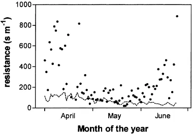
Crop surface resistance showed a seasonal trend with generally high values at the beginning and end of the period of growth and lower values in the middle, although there was considerable variability (Fig. 7). Two factors might be responsible for this pattern, green area index and soil water deficit.
For low values of GAI, rs should be inversely pro-portional to GAI since it can be estimated by summing
Fig. 7. Seasonal trend of linseed aerodynamic resistance (ra: dashed
line) and surface (canopy) resistance (rs: symbols). ra was
com-puted using the equation recommended in FAO 56, while rs was
in parallel the resistances for individual leaves above a representative area of ground. Fig. 8 plots rs against GAI for all dates when GAI was measured. The data points span the periods before and after the achieve-ment of maximum GAI but there was no evidence of hysteresis in the curve. The points are close to the line representing the relationship:
rs= rs min
G
where rs minis 90 s m−1and G is GAI.
The constant of proportionality, rs min,which is the surface resistance of an actively growing linseed crop completely covering the ground and freely supplied with water, was estimated, using the data in Fig. 7, as the average value of rs for DAS 69-75 (23 May–29 May), when the ground cover exceeded 0.80, the soil water deficit was relatively low and rain was not a complicating factor. The equation given above gives a value for rsof 45 s m−1at the maximum GAI recorded whereas Fig. 8 suggests that rsdoes not decrease once GAI exceeds 1.00. Thus, rs can be modelled as the higher of the values calculated from GAI and 90 s m−1. Before investigating the effect of soil water deficit on rs, it was necessary to ascertain whether periods of rain were complicating the interpretation since rs should be zero for wet foliage. Four occasions were
Fig. 8. Relationship between linseed surface resistance (rs) and
green area index (GAI). The rs values are shown only for the
days on which direct GAI measurements were carried out. rs
was derived from evapotranspiration (BREBS) measurements and inversion of the Penman–Monteith equation. The data are fitted by the line representing the relationshiprs=90/G, where G is GAI.
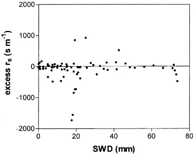
Fig. 9. Relationship between excess rs, defined as the measured
rs minus the modelled rs,calculated from GAI (green area index) with a minimum value of 90 s m−1, and the measured soil water
deficit (SWD) over the entire growing season.
found when a day on which more than 5 mm rain fell was both preceded and followed by a day with no significant rain. There was no consistent or significant difference between the values of rs on the three days and thus rainfall was not a factor having a main effect on surface resistance.
The effect of soil water deficit on rswas evaluated by computing the difference between the measured and the modelled rs and plotting it against the mea-sured soil water deficit (Fig. 9). The values of GAI required by the model were estimated by linear inter-polation between the field measurements. Contrary to expectations, there was no effect of SWD on surface resistance. This is particularly obvious for deficits ex-ceeding 50 mm where any affect should be clear. The apparent decrease of resistance at high deficits is prob-ably an artefact caused by an underestimate of GAI near crop maturity and the extreme sensitivity of rsto GAI at values of GAI near zero.
4. Discussion
apparently identical BREBS were used, they yielded rather different daytime evapotranspiration values on some occasions even after suspect values had been re-moved. It is possible that the threshold value used to discard data when the fetch was insufficient (20:1) was inadequate and although Heilman and Brittin (1989) showed that this limit was appropriate in their situ-ation, more conservative fetch values should perhaps have been used. Our data on the insignificance of night-time evapotranspiration are consistent with those of Malek (1992). He found that in a semi-arid environ-ment, although night-time evapotranspiration from an alfalfa (Medicago sativa L.) crop could reach 14% of the 24 h average under conditions of high windspeed at night (i.e. reaching 5 m s−1) the growing season av-erage was less than 2%. During the growing season only six nights had average windspeeds that exceeded 2 m s−1. Night-time evapotranspiration was thus not significant in the present work.
The difference between the calculated and measured SWDs in the earlier phase of growth can be explained by errors in the estimation of profile available water. After day 60, the measured SWD underestimated the calculated value. During this period, the soil did not return to field capacity and drainage from the profile is unlikely. However, the measurement of SWD was unable to take into account the removal of water from the layer between 0.60 m and the base of the root-ing zone. Although the maximum SWD exceeded the calculated profile available water, the discrepancy can be explained by the use of−0.03 MPa to assess field capacity. Webster and Beckett (1972) found that the matric potential of well-drained soils at field capacity was only about−0.005 MPa. Although these measure-ments were made in England during winter when the low soil temperature would have resulted in greater surface tension and viscosity of the water than in Italy in summer, the appropriate matric potential is likely to have been nearer the latter than the former, thus leading to an underestimate of available water.
Analysis of the surface resistance data was com-plicated by its variability. A sensitivity analysis was carried out to establish the effect of a±20% change in daily evapotranspiration (Ea) on surface resistance (c.f. Fig. 2). Decreasing Ea by 20% increased rs typi-cally by less than 10% but occasionally by up to 30%. Increasing Ea typically resulted in a decrease of 30 in but occasionally 100%. These errors, however, are
small compared with the seasonal trends and are un-likely to cause a systematic bias although they may go some way to explaining why the estimates are so variable.
not drought-stressed, glasshouse-grown linseed plants into the regression equation of Körner et al. (1979) and assuming a GAI of 1.0. This procedure gave a pre-dicted value for the minimum rs of 104 s m−1, which is consistent with the values calculated in the present paper, particularly, as glasshouse grown plants often exhibit a higher stomatal resistance than those grown in the field (Körner et al., 1979).
Other research has shown a positive relationship between rs and soil water deficit (e.g. Russell, 1980) caused by an increase of stomatal resistance in re-sponse to soil drying. In the present work, the soil effectively dried monotonically after DAS 60 and surface resistance showed the expected increase. However, the mechanism appears not to be through increased stomatal resistance of individual leaves but rather through canopy senescence. This observation may explain the overestimate of Kc adjobtained using the FAO 56 methodology (Section 3.3), which implic-itly assumes an effect on stomatal closure. Casa et al. (1999) similarly found that it was not drought as such that reduced linseed yield in Mediterranean conditions but rather the associated high temperatures which shortened the growth cycle and thus hastened canopy senescence. Linseed seems to be well adapted to avoid drought in an environment characterised by a summer drought, a phenomenon that may be more widespread in Mediterranean environments than is generally realised.
5. Conclusions
Although the Bowen ratio technique is typically employed for short periods of time because of the difficulties associated with instrument maintenance and missing data, it can also be successfully used in studies of seasonal crop water use. Daytime evapo-transpiration can be satisfactorily calculated for en-vironmental conditions similar to those encountered here, assuming a constant evaporative fraction and negligible night-time evaporation.
The total seasonal evapotranspiration of this spring-sown linseed crop was shown to be about 240 mm. Even taking into account that the crop was water-stressed for part of the time, linseed water re-quirements are thus rather modest compared with the other crops.
The agreement between the measured crop coeffi-cients and those obtained using the FAO 56 method-ology was good, considering that daily estimates were compared. In the initial growth stage, the FAO 56 method seemed to overestimate evaporation following rain events. When much of the available water ap-peared to have been used up in the final part of the growing season, measured Kcexceeded the values ad-justed for water stress. This is probably caused by an underestimate of the water in the soil at field capac-ity. Overall, however, the crop coefficients for linseed tabulated in FAO 56 seem appropriate for the environ-mental conditions of central Italy.
The determination of the factors affecting the sur-face resistance of the canopy was complicated by the variability of the estimates. However, the surface resistance was inversely related to GAI when GAI was less than 1.00 and was 90 s m−1when GAI was greater than 1.00. There was no consistent direct effect of soil water deficit on surface resistance although dry conditions hastened senescence and thus increased rs indirectly. These results could help improve the link between the crop coefficient and Penman–Monteith approaches to estimating crop evapotranspiration.
Acknowledgements
The authors would like to thank professor J.L. Monteith for his helpful comments on the manuscript. We also wish to thank Dr. R.G. Allen for reading the manuscript and for his valuable suggestions and M. Smith from FAO who kindly provided a draft copy of the FAO 56 paper. This work was carried out in the framework of the PRISCA programme of the Italian Ministry of Agricultural Policy.
References
Allen, R.G., Pereira, L.S., Raes, D., Smith, M., 1998. Crop eva-potranspiration — guidelines for computing crop water require-ments. FAO Irrigation and Drainage, Paper no. 56, Rome, Italy. Allen, R.G., Smith, M., Perrier, A., Pereira, L.S., 1994. An update for the definition of reference evapotranspiration. ICID Bull. 43, 1–34.
Angus, D.E., Watts, P.J., 1984. Evapotranspiration — how good is the Bowen ratio method? Agric. Water Manage. 8, 135–150. Blake, G.R., Hartge, K.H., 1986. In: Klute, A. (Ed.), Methods of soil analysis. ASA-SSSA, Agronomy Monograph, 9, 363–375. Casa, R., D’Antuono, L.F., Rossini, F., 1997. Simulazione della produzione potenziale del lino da olio (Linum usitatissimum L.) mediante il modello SUCROS. Applicazioni preliminari. Rivista di Agronomia 31, 624–633.
Casa, R., Russell, G., Lo Cascio, B., Rossini, F., 1999. Environmental effects on linseed (Linum usitatissimum L.) yield and growth of flax at different stand densities. Eur. J. Agron. 11, 267–277.
Choisnel, E., de Villele, O., Lacroze, F., 1992. Une approche uniformisée du calcul de l’évapotranspiration potentielle pour l’ensemble des pays de la Communauté Européenne. EUR 14223, Office des Publications Officielles des Communautées Européennes, Luxembourg.
Doorenbos, J., Pruitt, W.O., 1977. Crop water requirements. FAO Irrigation and Drainage, Paper no. 24, Rome, Italy, 144 pp. Dutta, H.K., Ram Mohan Rao, D.S., Singh, H., 1995. Response
of linseed (Linum usitatissimum L.) to irrigation and nitrogen. Indian J. Agron. 40, 130–131.
Grattan, S.R., Bowers, W., Dong, A., Snyder, R.L., Carroll, J.J., 1998. New crop coefficients estimate water use of vegetables, row crops. California Agric. 52, 16–21.
Gupta, R.K., Agrawal, G.G., 1977. Consumptive use of water by gram and linseed. Indian J. Agric. Sci. 47, 22–26.
Hanks, R.J., 1985. Crop coefficients for transpiration. In: Advances in Evapotranspiration. Proceedings of National Conference on Advances in Evapotranspiration, Chicago, ASAE, St. Joseph, MI, USA, pp. 431–438.
Heilman, J.L., Brittin, C.L., 1989. Fetch requirements for Bowen ratio measurements of latent and sensible heat fluxes. Agric. For. Meteorol. 44, 261–273.
Hsiao, T.C., Henderson, D.W., Matson, C., Held, A., Wranovics, C., Seymour, V., 1985. Improvement of crop coefficients for evapotranspiration. CIMIS Final Report, Vol. 1, Department of L.A.W.R., University of California, Davis, CA, USA, pp. 3–35. Howell, T.A., Steiner, J.L., Schneider, A.D., Evett, S.R., 1995. Evapotranspiration of irrigated winter wheat — southern high plains. Trans. ASAE 38, 745–759.
Jagtap, S.S., Jones, J.W., 1989. Stability of crop coefficients under different climate and irrigation management practices. Irrig. Sci. 10, 231–244.
Jarvis, P.G., McNaughton, K.G., 1986. Stomatal control of transpiration: scaling up from leaf to region. Adv. Ecol. Res. 15, 1–49.
Körner, C., Scheel, J.A., Bauer, H., 1979. Maximum leaf diffusive conductance in vascular plants. Photosynthetica 13, 45–82. Lull, H.W., 1964. Ecological and silvicultural aspects. In: Chow,
V.T. (Ed.), Handbook of Applied Hydrology, 6.9–6.10. McGraw Hill, New York, NY, USA.
Malek, E., 1992. Night-time evapotranspiration vs. daytime and 24 h evapotranspiration. J. Hydrol. 138, 119–129.
Malek, E., 1993. Rapid changes of the surface soil heat flux and its effects on the estimation of evapotranspiration. J. Hydrol. 142, 89–97.
Malek, E., Bingham, G.E., 1993. Comparison of the Bowen ratio-energy balance and the water balance methods for the measurement of evapotranspiration. J. Hydrol. 146, 209–220. Monteith, J.L., 1965. Evaporation and environment. In: Fogg, G.E.
(Ed.), The State and Movement of Water in Living Organisms. Symposium XIX of the Society for Experimental Biology, Cambridge University Press, Cambridge, UK, pp. 205–234. Ohmura, A., 1982. Objective criteria for rejecting data for
Bowen-ratio flux calculations. J. Appl. Meteorol. 21, 595–598. Pruitt, W.O., 1991. Development of crop coefficients using lysimeters. In: Allen, R.G., Howell, T.A., Pruitt, W.O., Walter, I.A., Jensen, M.E. (Eds.), Proceeding of the ASCE International Symposium on Lysimetry, Honolulu, HA, ASCE, New York, NY, USA.
Ritchie, J.T., 1972. Model for predicting evaporation from a row crop with incomplete cover. Water Resour. Res. 8, 1204–1213. Ritchie, J.T., Johnson, B.S., 1990. Soil and plant factors affecting evaporation. In: Stewart, B.A., Nilsen, D.R. (Eds.), Irrigation of Agricultural Crops. Agronomy series, 30, A.S.A., pp. 363–390. Rode, J.C., Bethenod, O., 1980. Influence de la carence hydrique sur le comportement photosynthétique du lin. Ann. Agron. 31, 285–295.
Russell, G., 1980. Crop evaporation, surface resistance and soil water status. Agric. Meteorol. 21, 213–226.
Smith, M., Allen, R.G., Monteith, J.L., Perrier, A., Pereira, L., Segeren, A., 1992. Report on the expert consultation on procedures for revision of FAO guidelines for prediction of crop water requirements. UN-FAO, Rome, Italy, 54 pp. Sinclair, T.R., Allen, J.R., Lemon, E.R., 1975. Analysis of errors
in the calculation of energy flux densities above vegetation by a Bowen ratio profile method. Boundary Layer Meteorol. 8, 129–139.
Stannard, D.I., 1997. A theoretically based determination of Bowen ratio fetch requirements. Boundary Layer Meteorol. 83, 375– 406.
Steven, M.D., Biscoe, P.V., Jaggard, K.W., Paruntu, J., 1986. Foliage cover and radiation interception. Field Crops Res. 13, 75–87.
Sugita, M., Brutsaert, W., 1991. Daily evaporation over a region from lower boundary layer profiles. Water Resour. Res. 27, 747–752.
Tattari, S., Ikonen, J.P., Sucksdorff, Y., 1995. A comparison of evapotranspiration above a barley field based on quality tested Bowen ratio data and Deardoff modelling. J. Hydrol. 170, 1–14. Tiwari, K.P., Dixit, J.P., Saran, R.N., 1988. Effect of nitrogen and irrigation on linseed (Linum usitatissimum L.). Indian J. Agron. 33, 44–46.
Vetter, H., Scharafat, S., 1964. Die wurzelverbreitung landwirtschaftlicher kulturpflanzen im unterboden. Z. Acker-u Pfl. Bau 120, 275–298.
Webster, R., Beckett, P.H.T., 1972. Matric potentials to which soils in south central England drain. J. Agric. Sci. Camb. 78, 379–387.
Wright, J.L., 1982. New evapotranspiration crop coefficients. J. Irrig. Drain. Div., ASCE 108 (IR2), 57–74.