Measurements of CO2
and energy fluxes over a mixed hardwood
forest in the mid-western United States
Hans Peter Schmid
∗, C. Susan B. Grimmond, Ford Cropley, Brian Offerle, Hong-Bing Su
Department of Geography, Indiana University, Bloomington, IN 47405, USAReceived 28 June 1999; received in revised form 13 March 2000; accepted 14 March 2000
Abstract
Results from the first full year of measurements (1998–1999) of above canopy CO2and energy fluxes at the AmeriFlux
site in the Morgan-Monroe State Forest, IN, USA, are presented. The site is located in an extensive secondary successional broadleaf forest in the maple-beech to oak-hickory transition zone. The minimum fetch is 4 km. Turbulent flux measurements are obtained by an eddy-covariance system at 46 m (1.8 times the canopy height) with a closed-path infrared gas analyzer.
Peak vegetation area index (VAI) was determined as 4.7±0.5 and the mean albedo during the vegetative period was 0.15±0.02. The aerodynamic roughness length was estimated as 2.1±1.1 m. It showed little variation with wind direction or season. The seasonal variations of energy partitioning and of net CO2exchange are discussed in terms of the phenological
development of the forest. To estimate the annual net ecosystem production (NEP) and carbon sequestration, eddy-covariance measurements during periods of poorly developed turbulence at night, and missing data were replaced by a simple parametric model based on measurements of soil temperature and photosynthetically active radiation (PAR). The night-time flux correction reduces the annual sequestration estimate by almost 50%. The corrected estimate of annual NEP for the 1998–1999 season is 2.4 t C ha−1per year±10%. © 2000 Elsevier Science B.V. All rights reserved.
Keywords:AmeriFlux; Forest-atmosphere exchange; Eddy-covariance; Carbon sequestration; Forest micrometeorology
1. Introduction and background
This paper presents the first set of results (March 1998–February 1999, inclusive) from a long-term project measuring forest-atmosphere exchanges of
CO2, water vapor and energy balance components
over the Morgan-Monroe State Forest (MMSF), a mixed deciduous forest in south-central Indiana in the mid-western United States.
The central objective of this research is to en-hance empirical and theoretical understanding of
∗Corresponding author. Tel.:+1-812-855-6303; fax:+1-812-855-1661.
E-mail address:[email protected] (H.P. Schmid)
soil-vegetation-atmosphere exchanges of carbon diox-ide, and associated fluxes of water vapor, radiation and heat. With only a few direct long-term mea-surements of terrestrial carbon exchange available, these estimates are virtually unconstrained by reliable benchmark values (Baldocchi et al., 1996, and other papers in the same special issue). If, as the ‘missing sink’ argument implies (Tans et al., 1990; Ciais et al., 1995; Schimel, 1995), mid-latitude forests play an important role in global carbon sequestration, its causes, dynamics, and future trends are unknown, leaving the potential for error in predictions of future atmospheric CO2concentrations wide open. Recently,
the attribution of the missing sink to mid-latitude forests has gained support by linking satellite-inferred
increases in normalized difference vegetation index (NDVI) over the period 1981–1991 to net increases in biomass (Myneni et al., 1997). Another study re-ported an annual carbon sink over the north-eastern United States that alone accounts for the global miss-ing sink, based on the carbon mass-balance inversion method for 1988–1992 (Fan et al., 1998). While these studies provide invaluable information about the mag-nitudes involved in the global carbon cycle, the large uncertainties in their results point to the deficiency of current knowledge about terrestrial carbon exchanges. These concerns formed the basis for the establish-ment of long-term carbon flux networks in Europe (Euroflux, Valentini et al., 1996) and in the Amer-icas (AmeriFlux, Wofsy and Hollinger, 1997). To-gether with other emerging networks in Australia and Asia, these efforts are coordinated by FLUXNET (Baldocchi et al., 1998). The flux measurements at MMSF, described in this study, are part of the Amer-iFlux network and became operational in February 1998. This project concentrates on micrometeoro-logical aspects of forest-atmosphere exchange. It is closely associated and complemented by partner projects on ecosystem responses to carbon exchange, and on carbon–nitrogen relations (Pryor et al., 1998; Randolph, 1998).
To gain process level knowledge on forest-atmos-phere exchange of carbon dioxide, it is necessary to recognize the linkages between the exchange of car-bon, water vapor, heat and radiation. In this paper, we discuss daily and seasonal variations of exchanges of energy and carbon dioxide using the framework of the surface energy balance equation
Q∗=QH+QE+QG+1QS+QP (1) whereQ∗ is the net radiation,QH andQE the fluxes
of sensible and latent heat, respectively, QG the soil
heat flux,1QS the heat storage change in the canopy
volume andQPis the energy fixed by photosynthesis),
and a simplified form of the ecosystem carbon balance equation
NEP=GEP−RE= −(FCO2+1CS) (2)
where NEP is the net ecosystem production, GEP the gross ecosystem production due to photosynthesis mi-nus plant respiration,RE the total ecosystem
respira-tion,FCO2 the net flux of carbon dioxide and1CS is
the carbon storage change in the volume. The symbol QEand the term ‘evaporation’ are used synonymously
with ‘evapotranspiration’. For atmospheric fluxes, the usual sign convention, positive upward, is used. Thus,
net ecosystem exchange, NEE=−NEP.
A detailed description of the methods and locations of measurement used for individual terms of these bal-ance equations is given in Section 2. Data for time periods when measurements are missing due to pre-cipitation, instrumentation problems or conditions in which the eddy covariance method becomes question-able for measuring the flux exchange (e.g., extremely weak turbulence in the stable boundary layer during calm nights) are interpolated using a simple paramet-ric model, based on measurements of soil temperature and photosynthetically active radiation (PAR) (Section 4.3). Additional complications are introduced by the presence of topography and ensuing mean vertical flow components. Questions and concerns about the con-sequences of vertical mean flow, advection and insta-tionarity on the form of the conservation of mass equa-tion are addressed by Lee (1998), Paw U et al. (1998) and Finnigan (1999). The estimates from this study of annual carbon sequestration (net ecosystem produc-tion), annual gross ecosystem production and annual ecosystem respiration are discussed in terms of the magnitudes, uncertainties, and inter-annual variability found at other mid-latitude broad-leaf forest sites.
2. Site and instrumentation
MMSF, south-central Indiana (39◦19′N, 86◦25′W),
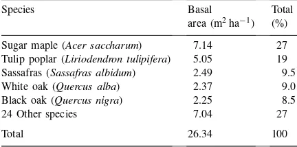
Table 1
Species composition of tree basal area of MMSF from 54 large plots surrounding the study site covering a total of 8100 m2. Total
above ground biomass was determined as 19.52 kg m−2 (Ehman,
personal communication)
Species Basal Total
area (m2ha−1) (%)
Sugar maple (Acer saccharum) 7.14 27 Tulip poplar (Liriodendron tulipifera) 5.05 19 Sassafras (Sassafras albidum) 2.49 9.5
White oak (Quercus alba) 2.37 9.0
Black oak (Quercus nigra) 2.25 8.5
24 Other species 7.04 27
Total 26.34 100
black oak (Quercus nigra) (Table 1). The mean canopy height of the forest is≈25–27 m. This forest is located just south of the limit of the Wisconsinan glaciation.
The study site is located so that the minimum fetch of essentially uninterrupted forest exceeds 4 km in any direction, and reaches up to 8 km in the principal wind
Fig. 1. Map of the MMSF tower site. Contour interval is 10 ft (3.05 m).
direction (westerly to south-westerly). The principal site for flux measurements is a 46 m meteorological tower (Fig. 1), which is accessed via a non-public road. These measurements are augmented by four microm-eteorological stations below canopy in the expected footprint of the tower.
acquisition equipment, the gas flow control system, and the Infra-red gas analyzers (IRGAs, Li-6262 from LiCor, Lincoln, NE).
The micrometeorological instrumentation is orga-nized into two main observation levels for flux mea-surements on the tower (at 46 and 34 m) and one on a separate mast below canopy (at 1–2 m). The latter is
≈10 m to the southwest of the tower, to avoid the dis-turbance in the canopy structure created by the tower (see Table 2 for a summary of all instrumentation). At each of these levels the four components of the radi-ation balance are measured separately, along with net all wave radiation (Q∗), and sensors for PAR are lo-cated at 46 m, at 22 m (≈80% of canopy height), and at 2 m, below canopy. Total incoming shortwave radi-ation (K↓) is also measured at approximately canopy height (28 m), in mid-canopy (14 m), and again at 2 m, to complete a six level profile of incoming shortwave radiation (K↓or PAR) through the canopy.
Measurements of three dimensional turbulent velocity fluctuations and eddy-covariance fluxes of
Table 2
Instrumentation for continuous micrometeorological observations at the MMSF towera
Measurement Manufacturer Instrument
Fluxes
46, 34, 2 m 3D Wind, eddy-covariance CSI, Logan, UT CSAT
46, 34, 2 m CO2and H2O, eddy-covariance LiCor, Lincoln, NE Li-6262
46, 34, 2 m Four component net radiation Kipp and Zonen, Bohemia, NY CNR1
46, 34, 2 (4×) m Net radiation REBS, Seattle, WA Q∗7/Q∗6
28, 14, 2 (4×) m Incoming short wave LiCor, Lincoln, NE Li-200SZ-50
46, 22, 2 (4×) m PAR LiCor Lincoln, NE Li-190SZ-50
Profiles
32, 16, 8, 4, 2, 1, 0.5, 0.25 m CO2and H2O, mean profile LiCor Lincoln, NE Li-6262
(32×) Bole temperature Omega, Stamford, CT T-type
46, 34, 22, 12, 6, 1 m Air temperature and relative humidity Vaisala (sensors), Woburn, MA HMP35C R.E. Young (shields), Traverse City, MI (Aspirated) Auxiliary
0 m Barometric pressure Vaisala, Woburn, MA PTA 427
46, 0 (4×) m Precipitation Texas Electronics, Dallas, TX TE525
Qualimetrics, Sacramento, CA 6011-B
3 m Snow depth CSI, Logan, UT SR-50
Soil
(6×) Surface wetness CSI, Logan, UT 237
(4×) Soil moisture CSI, Logan, UT CS615
(4×) Soil temperature Omega, Stamford, CT T-type
(4×) Soil temperature CSI, Logan, UT TCAV
(8×) Soil heat flux plates REBS, Seattle, WA HFT
aMultiple sensors distributed in the study area are indicated by their number (e.g., 4×or 32×).
momentum, sensible heat, water vapor, and CO2
are also obtained at 46, 34, and 2 m. At the two above-canopy levels, the azimuth orientation of
the sonic anemometers is 230◦. The fluxes of
mo-mentum and heat are evaluated directly from the three-dimensional sonic anemometers (CSAT, Camp-bell Scientific Inc. (CSI), Logan, UT, 10 Hz sampling
rate). The water vapor and CO2 concentrations are
measured by pumping sample air from the three sonic anemometer levels to individual closed-path IRGAs inside the shelter. Eddy-covariance fluxes are then obtained during post-processing (Section 3).
These flux levels are augmented by profile measure-ments of CO2, air temperature and relative humidity
at multiple levels above and throughout the canopy.
Detailed profiles of water vapor and CO2 mixing
trees, so that they are located within undisturbed canopy space. Air temperature and humidity profiles are provided by six levels of combined ventilated T/RH probes along one leg of the tower (Table 2). To evaluate the heat storage dynamics of tree trunks and boles in the canopy volume, a number of trees of various species and stages of maturity have been equipped with bole temperature sensors. These pro-file measurements form the basis for the evaluation of the canopy volume storage terms of heat and CO2
in Eqs. (1) and (2). All these variables are sampled at 10 Hz and pre-processed by a National Instruments Inc. (Austin, TX) data acquisition unit with LabView software.
Below-canopy conditions are examined by four mi-crometeorological stations distributed within the ex-pected footprint of the tower measurements. Variables measured at these stations includeQ∗, PAR, soil mois-ture, soil temperamois-ture, soil heat flux (QG), and
precip-itation. At the main below-canopy station (co-located with the 2 m eddy-covariance station), surface wetness and snow depth also are measured. The other three micrometeorological stations are co-located with three of the ecological plots (Fig. 1). These micrometeoro-logical variables are sampled at 5 s and averaged to 30 min by CSI 21X data loggers.
3. Eddy-covariance data acquisition and processing
3.1. Overview
The main instruments used for the eddy-covariance system are a CSAT 3-D sonic anemometer and an IRGA for each level (Table 2). Sample gas is pumped from the intake near the sonic anemometer array to the IRGA through Teflon tubing with an inner diame-ter of 4.8 mm. The total line length for the 46 m mea-surement level amounts to nearly 60 m. Inline Teflon filters (Gelman Inc., pore size=1mm) near the gas in-take prevent dust and dirt from entering the tubing. Heating tape, applied to the tubing on both sides of the filters and to the filters themselves, prevents the pressure drop associated with filtration from causing condensation. Inside the shelter, another section of the Teflon tubing is heated to damp out temperature fluc-tuations in the gas, and to allow the IRGAs to operate
at conditions of constant temperature. A further filter in the tubing immediately before the IRGA intake pro-tects the optical bench of the IRGA from any resid-ual contamination. On the exhaust side of the IRGA, the flow rate is monitored by a mass flow controller (GFC-17S, Aalborg Inc., Orangeburg, NY). This is connected in turn to a diaphragm pump, after passing through a dead volume, to dampen out vibrations from the pumps. The flow rate is approximately 7.5 l min−1,
leading to a Reynolds number of the flow of around 2300, just above the turbulence limit. The transit time for the 60 m tubing is on the order of 6 –7 s.
3.2. IRGA and eddy-correlation data processing
Calibration of the gas analyzers against gas stan-dards that are traceable to the National Institute of Standards is done at sampling pressure and flow rate to reduce the dependence upon the corrections applied using the IRGA’s internal pressure transducer cell. A system of solenoid valves enables gas cylinders for IRGA calibration to be permanently connected: the fixed connections decrease the susceptibility of the system to contamination by leaks. One solenoid valve in each of the sample lines switches between ‘line gas’ (from the tower) and calibration gas, which derives from a manifold. A second solenoid valve controls the flow of nitrogen gas or calibration standard CO2 to
the manifold. Needle valves allow adjustment of flow and pressure conditions in the IRGA to be identical to measurement conditions. Valve settings need to be set manually when gas cylinders are exchanged. A set of (electrical) switches allows this system to be operated either manually or automatically by the logging sys-tem in a scheduled manner. Currently, the calibration system cycles over the four IRGAs automatically ev-ery 27 h, so that the time of day for the calibrations is incremented daily. Automatic calibrations monitor but do not alter the IRGA instrument calibration. A span gas for water vapor calibration is not available at high enough flow rate. It is our intention that H2O span
calibration be done by reference to a calibration hu-midity probe on the tower near the gas intake, though currently this is not done, except by weekly compari-son with psychrometer readings.
Raw voltage values (mV) of CO2, H2O, sample
and H2O are then calculated following the procedures
described in the manual of Li-6262 and calibration co-efficients specific for each IRGA. These include the dilution correction due to water vapor (Webb et al., 1980). Eddy-covariance fluxes are calculated by shift-ing the time series of the gas concentration and ver-tical velocity to maximize the correlation coefficient between them. A first guess for the lag window is pro-vided by the flow rate and the tube dimensions.
Detection and rejection of data spikes is achieved during data processing of both the IRGAs and the sonic anemometers, using a conservative approach. Some spikes are indicated by a flag variable in the CSAT output, indicating problems, such as a blocked path between a sensor pair. Such flagged spikes can generally be attributed to precipitation. Following Vickers and Mahrt (1997), we call these ‘hard’ spikes and unambiguously reject the corresponding periods of CSAT data. This is a conservative policy as some of the CSAT flag values indicate that the data is merely suspect and not unusable outright.
A second type of spike, termed here ‘soft’ spikes because they are detected by post-processing crite-ria, are large short-lived departures from the (15 min) means, detected in an iterative process, similar to that described in Højstrup (1993) (although his model ap-plies to the time derivative of the signal). For each 15 min period and variable, the means and variances are calculated. From these diagnostics, a threshold for spikes is determined as a multiple of the standard de-viation, with the multiplier increasing on each iter-ation (3.6 S.D. initially, increased by 0.3 after each pass). On each pass, a soft spike is registered if the fluctuation from the mean is larger than the threshold value, and if the duration of the spike is three or fewer records, corresponding to a persistence of 0.3 s for the 10 Hz sampling rate. Longer-lasting departures from the period mean are taken to indicate possible physi-cal events. After each pass, if spikes are detected, the mean and variance are adjusted to exclude data marked as spikes and the process repeated, until either there are no more new spikes or the maximum of three it-erations is completed (which is rarely the case).
It was found that hard and soft spikes are closely related. The data appear to start to go out of range before the instrument’s self-diagnosis indicates a problem, which vindicates the decision to take a con-servative approach to data rejection. After this first
phase of quality control, eddy-correlation fluxes and other turbulence statistics are determined over periods of 15 min, if more than 50% of the raw data pass the spike rejection test for a given 15 min block. Other-wise, the entire block is treated as a missing value. Here, traditional Reynolds decomposition based on block averages is used, although this method requires an assumption of weak stationarity, which is unlikely to be strictly warranted in all conditions encountered during the study period (e.g., Paw U et al., 1998).
In a second phase of quality control, all measured or derived variables (15 min averages) are submitted to a plausibility test and are rejected if they fall out-side statically defined constraints for each variable (e.g., energy fluxes not to exceed the solar constant, CO2fluxes not to exceed±50mmol m−2s−1). Subse-quently, the 15 min data are reduced to hourly aver-ages. If more than one 15 min block in a given hour is missing, the entire hour is treated as a missing value. The use of three or four 15 min block averages for hourly fluxes over very rough surfaces is a strat-egy to minimize the need to reject data over a given measurement period. It is a compromise between including the peak frequencies of the co-spectrum and avoiding non-stationarity effects in longer aver-aging periods, but raises the question of unresolved flux contributions at periods longer than 15 min. On YD 98/175–177 (24–26 June 1998), a field com-parison of the present eddy-covariance configuration and the AmeriFlux roving standard system, using 30 min flux averages but similar tubing and flow rate, was carried out (Evans, personal communica-tions). For a description of the roving standard sys-tem, see http://cdiac.esd.ornl.gov/programs/ameriflux (Hollinger, personal communications). The results fully support the use of the present data management strategy. Measurements were conducted over a range of 12mmol m−2s−1≥FCO2≥−32mmol m−2s−1. The FCO2 values of the resident system at MMSF agreed
very closely with the roving standard, as demonstrated by the regression statistics. Based on 86 observations, the coefficient of determination R2, was 0.97 and the S.E. 1.8mmol m−2s−1. The MMSF system over-estimated the roving standard slightly, with a slope
of 1.08. For H2O, the comparison was even more
an underestimation of the flux, compared to using a 30 min window, but reduced the need to reject data considerably.
3.3. Frequency response of CO2 and H2O
measurements
Although the Li-6262 CO2/H2O IRGA allows a
10 Hz sampling rate, the actual frequency resolution of CO2 and H2O measurements is likely reduced by
any mixing or smearing of the sampled ambient air in the long tube of 60 m, through which the sam-ple air is pumped. To correct flux measurements for such tube attenuations, various methods have been suggested (e.g., Moore, 1986; Leuning and Moncrieff, 1990; Eugster and Senn, 1995; Leuning and Judd, 1996; Massman, 2000) with differing degrees of as-sumptions about the corrected shape of the spectrum. We consider this topic a research question that needs careful consideration where individual values of mea-sured fluxes are important. Here, we concentrate on relative magnitudes and argue that, for the present method to obtain an annual estimate of NEP, the effect of tube attenuation is small.
In samples of spectra from the measured CO2and
H2O time series (not shown), the −5/3 slope of the
inertial subrange only extends to a natural frequency of about 0.1–0.2 Hz, above which the spectral densi-ties decay with an increasing slope, and are reduced to the white noise level above 1 Hz (the actual IRGA resolution limit for our configuration). This finding is no surprise, because the tube acts as a low-pass filter and higher frequencies are attenuated more ef-fectively. The strength of this attenuation depends on the Reynolds number, on the tube diameter, the tube material and on its length. The residence time in the tube is approximately equivalent to the time constant of the tube attenuation characteristics (Eugster and Senn, 1995). As shown by Leuning and Moncrieff (1990), the relative magnitude of the flux loss due to tube attenuation depends upon the mean wind speed and measurement height, in addition to the tube attenuation characteristics.
However, for the present purposes of analyzing data from the 46 m level, spectral losses are considered minimal. This conclusion is reached, because (i) large organized coherent structures dominate the exchange over tall forest canopies (Shaw and Tavangar, 1983;
Raupach et al., 1986; Su et al., 1998) with a spatial length scale of 4–12 times canopy height (Zhang et al., 1992; Raupach et al., 1996; Su et al., 2000), and (ii) the eddy-covariance system at 46 m is relatively high, corresponding to about 1.8 canopy heights, so that the percentage of flux correction is expected to be small. For example, Leuning and Moncrieff (1990) showed that, for a mean wind speed range from 1 to 10 m s−1, flux loss ranged from 21 to 38% at 1 m
height, the corresponding loss for 8 m height is re-duced to between 4 and 8%. For our measurement height at more than 25 m above the displacement level, we expect substantial further reduction of this effect.
Our assessment of the minimal impact of tube attenuation for our experimental design and data treatment is confirmed indirectly by an independent estimate of annual NEP, from measurements of above and below ground biomass increments (Ehman et al., 1999), within 10% of the micrometeorological flux integration value, as presented in Section 5.
4. Results
4.1. Micrometeorological site characterization
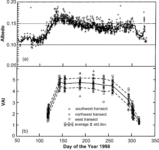
The albedo (a) of the tower site was determined with the up- and down-looking CNR1 pyranome-ters at 46 m (Fig. 2a). To avoid run-away ratios and low solar angles, only hourly couplets with incom-ing shortwave radiation,K↓>150 W m−2 were used.
Fig. 2. Forest phenology over the vegetative season of 1998 at MMSF. (a) Variation of albedo. Dots are hourly values and the solid line is a 10 day moving average. (b) Evolution of total VAI. See Fig. 1 for transect locations.
Total VAI was measured periodically at over 30 locations on three transects in south-western, north-western, and western direction, using a LiCor LAI-2000 sensor, with full sky reference measured at the top of the tower (Fig. 2b). The leaf-off bole area index was determined at about 1.3±0.16 on 13 November (98/317), after leaf fall. Unfortunately, adverse weather conditions in spring of 1998 pre-vented most VAI measurements during the budding period, starting in early April. Because the winter of 1997–1998 was unusually mild in this region (mostly attributed to the strong El Nino event during that pe-riod), the onset of budding was visually observed to be about 2 weeks earlier than usual (Randolph, per-sonal communication). The data show that this period was complete by 22 May (98/142), after which VAI
remained approximately constant at 4.7±0.5 until
98/217, at the beginning of August. In August and the first half of September, leaf senescence decreased the VAI to 4.48±0.4, and after that date (98/259) the foliage began to fall, as indicated by the steepening decrease of VAI down to its leaf-off value. The mag-nitudes and evolution pattern of VAI at the MMSF
site are very similar to those for the oak-hickory for-est at the Walker Branch AmeriFlux site near Oak Ridge, Tennessee, as reported by Huchison et al. (1986) and more recently by Greco and Baldocchi (1996), forthwith denoted as GB96 for the vegeta-tive season of 1993. Due to the latitudinal difference (Walker Branch is at 35◦57′N, 3◦22′ further south
than MMSF), we expect that the growing season at Walker Branch is typically longer than at MMSF, as direct phenological comparisons confirm (Baldocchi, 1999, personal communication).
To estimate the roughness length of the forest (z0), the hourly values of mean wind speed and
fric-tion velocity measured by the sonic anemometer at 46 m were used for near neutral conditions (where |L|>1000 m, andLis the Obukhov length) with wind speeds over 2 m s−1, in conjunction with the
loga-rithmic wind profile relation. It was assumed that the zero-plane displacement height, zd=0.8h, where
h is the mean canopy height of 26 m. Changing zd
to 0.75h affected the computed roughness lengths
with wind direction around the site, except for a narrow sector at about 50◦, where the apparentz
0
de-creases to nearly 1 m. Flow reaching the sensor from this sector comes across the broad ridge on which the tower is located (Fig. 1), but this sector also is aligned with the tower structure upwind of the sensor, thus flow conditions are very likely disturbed. There is no discernable seasonal variation between leaf off and leaf out periods. The use of the logarithmic wind pro-file relation is not a priori warranted here, because the 46 m level may be too low to be above the roughness sub-layer, where the logarithmic law does not apply. In addition, terrain induced flow features would need to be considered in a more exact analysis. However, the relatively well-behaved results (not shown) justify the use of this crude method for an estimate ofz0.
4.2. CO2and energy fluxes: daily and seasonal
variations
Despite the good agreement of the present eddy-covariance system with the AmeriFlux standard, the
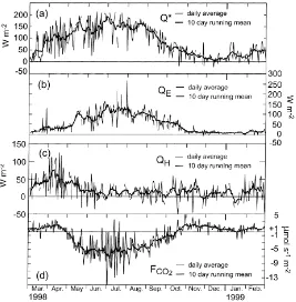
Fig. 3. Annual variation of energy and CO2 fluxes: (a) net radiation; (b) latent heat; (c) sensible heat and (d) CO2.
data available at this time do not allow detailed inter-pretations of the energy balance in the soil-canopy-air volume at this site, before some of the concerns associated with topographic effects and divergence, mentioned in the introduction can be addressed. In ad-dition, the spatial representativeness of the radiation and eddy-covariance footprints need to be examined (Schmid, 1997). Using the present data, and assuming that totalQGis small on an annual basis, the annual
to-tals ofQ∗−(Q
H+QE)=Q∗×17%. This lack of closure
is large, but comparable to similar studies (Blanken et al., 1998). Thus, our emphasis here is not on ab-solute values of energy fluxes, but on the diurnal and seasonal patterns.
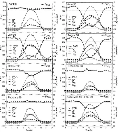
Because of their multiple links to the ecophysiol-ogy of the forest, the seasonal and diurnal patterns of radiation, sensible heat, evaporation and carbon fluxes need to be examined in concert. These results are presented in Figs. 3–5b. Even without complete confidence in the absolute levels ofQEandQH, Figs.
Fig. 4. Ensemble mean daily cycles of energy and CO2exchange for April, June, July, August, October, December 1998, February 1999,
and for the entire year.
QH follows the course ofQ∗closely in early spring,
it starts to decay drastically at the end of April and becomes almost completely decoupled from net ra-diation by the end of May. This occurs because of increasing latent heat transport, driven by transpira-tion from the emerging forest foliage. This trend is
reversed after leaf fall in October, whenQEdecreases
andQH once again becomes more significant to the
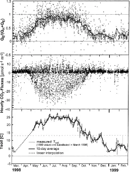
Fig. 5. (a) Annual course of day-time partitioning of convective energy at MMSF, 46 m level. Plus signs (+) are hourly ratios and the heavy line is a 10-day moving average. The dashed peaks indicate significant data gaps. (b) Annual composite of hourly CO2 fluxes measured
by eddy-covariance at 46 m above MMSF. Negative values indicate that the forest is a net sink of CO2. (c) Evolution of soil temperature
(at 5 cm) over the study period. Data for March and April 1998 are unavailable. The use of March 1999 data and an interpolation for the purposes of the GEP model is explained in the text.
the available energy is dominated by QE, while the
sensible heat flux exhibits only a weak diurnal pat-tern. Between mid-May and mid-September, about 85% of the day-time (K↓>100 W m−2) available
en-ergy is consumed by evaporation, in contrast to only around 20–30% during the leaf-off period (Fig. 5a). A comparison with Fig. 2b shows a strong correlation between energy partitioning and the development of VAI over the period. Grimmond et al. (2000) demon-strate that transpiration from trees and evaporation of intercepted precipitation by the forest canopy
con-tribute about 90% of the measured H2O flux above
canopy during the growing season. However, their
measurements indicate that evaporation of intercepted precipitation dominates transpiration by roughly 25%. The amount of PAR incident on the canopy, dur-ing the period when VAI is at its maximum, closely matches the amount of latent heat consumed during the day (Fig. 4). This relationship is quite distinct for June and July and to a lesser extent for August (August 1998 was very dry). Daily total evaporation at a similar forest site in the Walker Branch Water-shed, TN, reported by GB96 for the year 1993 shows similar magnitudes ofQEto the present study. On the
one summer day (YD 244, 1 September) reportedQE
that the forest exhibited signs of water stress during that time.
As expected, the close physiological link between leaf transpiration and the net exchange of CO2above
the canopy is expressed clearly both in the seasonal patterns and their diurnal course (Figs. 3 and 4). Neg-ative values ofFCO2 are directed towards the forest
and signify photosynthetic activity. Consistent with the rapid development of VAI in April and May, day-time negative CO2fluxes show a sharp gradient during this
period. While respiration is still dominant through-out the monthly mean day in April (Fig. 4), with hardly any organized diurnal pattern in the net flux, the forest has clearly become a net carbon sink in May (Figs. 3d and 5b). Fig. 3d shows that measured daily average respiration rates are low during most of winter. With warmer temperatures in April, respira-tion rates increase to result in net exchange of about 5mmol m−2s−1in the daily average, despite the onset of budding and photosynthetic activity. Peak positive hourly fluxes reach up to 10mmol m−2s−1during this period (Fig. 5b).
The scatter in Fig. 5b is an expression of the diurnal and seasonal courses ofFCO2, modulated by variations
in weather conditions that affectFCO2through changes
in the radiation balance, temperature, and moisture availability. However, small negative fluxes (and oc-casionally substantial ones) were obtained throughout the leaf-off period. This finding is consistent with the experience of other long-term flux observation sites over deciduous forests (e.g., GB96; Goulden et al., 1996a, forthwith G96). The persistence in the occur-rence of the smaller negative values in Fig. 5b, and the relatively large magnitude of the episodic ones during the period when photosynthesis is absent, suggests that these measurements cannot simply be attributed to instrument error. For this reason, they are not a priori rejected in our estimates of net ecosystem exchange (see below). The attempt to partition these values into
instrumental errors and CO2 storage change in the
soil-canopy-air volume beneath the tower, due to, for example, topographically induced episodic horizontal divergence, is a research question that will be pursued elsewhere. The short term and episodic nature of these negative fluxes is confirmed by the fact that they usu-ally disappear in the monthly averages for the leaf-off period (Fig. 4). In December 1998 and February 1999, there is a hint of a diurnal pattern of increased
respiration rates around noon, whereas the beginning of photosynthesis is hinted at by the slight reduction of net exchange during mid-day in April 1998.
4.3. Annual net carbon exchange and a simple model
In principle, eddy-covariance measurements of
FCO2 at 46 m (∼1.8 canopy heights) provide
di-rect measurements of the net ecosystem production or exchange (NEP or NEE) over the course of the study period. The ensemble of hourly observations of net ecosystem exchange is shown in Fig. 5b. Net ecosystem production can be formulated as a balance of gross ecosystem production (GEP, consisting of carboxylation, photorespiration and dark respiration; Farquhar et al., 1980), ecosystem respiration (RE),
and storage change.
The integral quality of the NEP observations pre-sented in this study can be assessed by examining this balance based on some first-order assumptions for a given ecosystem
1. GEP is dominated by photosynthesis and is pri-marily controlled by the photosynthetically active photon flux density (PPFD) or PAR received dur-ing the vegetative period;
2. The length of the vegetative season is the period over which the soil temperature (Ts) rises above a
certain threshold levelTsc;
3. Ecosystem respiration is largely controlled by the soil temperature; and
4. For extended periods of a few days to years, storage change of gaseous carbon dioxide in the soil-air volume beneath the tower is negligible.
The last assumption requires that, on an annual basis
NEPa= −
Z a
FCO2dt =GEPa−REa (3) in modification to Eq. (2), where the subscript ‘a’ refers to annual.
The above assumptions give rise to a very simple model for NEP
NEP=GEP(PPFD, Ts|Ts> Tsc)−RE(Ts) (4)
Once suitable relationships for GEP andREhave been
The annual course of soil temperature is presented in Fig. 5c. Unfortunately, soil temperature was not available before May 1998. For this reason, the first 10-days of March 1999 values were used in con-junction with a linear interpolation up to the first measured values during the study period, to sup-ply soil temperatures to be used in the model. To obtain a relationship between respiration and soil temperature, measured values ofFCO2 from the 46 m
eddy-covariance system during the period when the canopy was not fully developed or off-leaf were used (excluding Days 98/142–259). This method is similar to that suggested by Wofsy et al. (1993) ex-cept that they used eddy-fluxes corrected for storage change which are not available for this site yet. To compensate for this, a criterion for the measured friction velocity u∗>0.5 ms−1 was applied to ensure
well-developed turbulence and mixing between the sensor level and the soil surface. This criterion for u∗ is more conservative than those suggested by G96
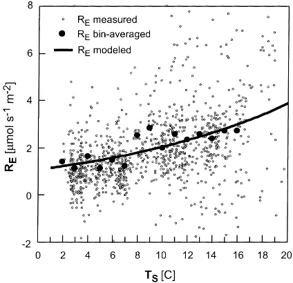
and Black et al. (1996) to exclude periods of intermit-tent turbulence, where the eddy-covariance technique becomes invalid. Based on chamber measurements and above-canopy eddy-covariance at Harvard Forest, Wofsy et al. (1993) determined that more than 80% of respiration is attributable to below-ground respira-tion (soil and root). Because the scatter in the results (Fig. 6) is very strong, the data were averaged in bins of 1◦C width. An exponential function, similar to those proposed by the studies mentioned above (and others), was fitted to the bin-averages
RE=1.08 exp(0.064Ts) (5)
where the fluxes are in mmol m−2s−1, andTs is in ◦C. The strength of the linear relationship between
modeled and observed fluxes (not the bin-averages) is expressed by a coefficient of determination (R2)
Table 3
Q10values obtained for broadleaf forests (ordered by increasing value)
Forest Location Latitude Source Temperature Q10
Oak-hickory Walker Branch, TN 36◦N GB96 Air 1.62
Maple-tulip poplar Morgan-Monroe, IN 39◦N Present study Soil 1.89
Oak-maple Harvard forest, MA 42.5◦N G96 Soil 2.1
Beech Central Italy, 1564 m a.s.l. 42◦N Valentini et al. (1996) Air 2.17 Hardwood forests Average worldwide N/A Kicklighter et al. (1994) Soil 3.08 Boreal aspen Prince Albert, Sask., CDN 53.7◦N Black et al. (1996) Soil 5.4
Fig. 6. Ecosystem respiration vs. soil temperature. The model (solid curve) fitted to the bin-averages is given in Eq. (5). (R2=0.66).
of 0.66 (n=1111). The correspondingQ10coefficient,
the factor by which respiration increases with a rise of 10◦C in soil temperature, is 1.89. This value lies well within those reported by various authors for other broadleaf forests (Table 3). Considering that the beech forest of Valentini et al. (1996) lies at an altitude of 1564 m a.s.l., Table 3 suggests a positive latitudinal trend ofQ10estimates for hardwood forests.
As postulated in Assumption (2), photosynthesis is fully active during a period whenTsremains above a
certain thresholdTsc. A comparison of Figs. 2b and 5a
and b with Fig. 5c supports this assumption and sug-gests a threshold temperature ofTsc=13◦C, resulting
1998. The same threshold temperature phenomenon, near the climatological average soil temperature, was observed also at other forests and for other years by Baldocchi (1999, personal communication). This find-ing suggests that the climatological average soil tem-perature may serve as a physiological or biochemical trigger for the vegetation.
Although Eq. (5) was obtained for a small subset of flux measurements (based on 12.7% of the data, see above), it was used to estimate gross ecosystem pho-tosynthesis or GEP during day-time (PPFD>0), over the entire period when VAI was fully developed (from 22 May–16 September, 98/142–259, Fig. 2b), as the difference betweenFCO2−RE, where RE is obtained
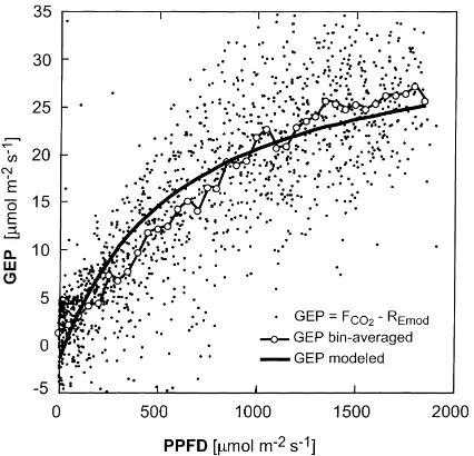
by Eq. (5). When the data are averaged to bins of 50mmol m−2s−1 of PPFD, the trend unrealistically shows no saturation at high PPFD (Fig. 7). Thus, the functional relationship fitted to the data was not al-lowed to adjust in a free regression. Instead, a similar equation to that used by G96 was used, allowing for saturation at higher PPFD values
GEP= −1.4+35× PPFD
590+PPFD (6)
where the fluxes are in mmol m−2s−1. With Eq. (6) the maximum photosynthetic rate is estimated to be
Fig. 7. GEP vs. PPFD. The model (smooth solid curve) is given in Eq. (6). (R2=0.65).
slightly higher than at Harvard Forest (G96) and slightly lower than the theoretical optimum values for broadleaf forests proposed by GB96. The coefficient of determination between ‘observed’ and modeled GEP values using Eq. (6) is 0.65 (n=1466). In reality, this strong physical relation between radiation and photosynthesis is modulated by environmental factors affecting the vegetation, such as water stress and leaf area index (e.g., GB96), but these factors are ignored here.
Ecosystem respiration given by Eq. (5) was used to correct the net ecosystem CO2 fluxes obtained by
eddy-covariance during calm nights, when turbulence is not well developed or drainage effects may influ-ence the measurements. In addition, the combination of Eqs. (4)–(6) was used to fill the data gaps in the
FCO2 time series over the entire study period. The
cu-mulative NEE over the year (Fig. 8), arbitrarily starting at zero at the beginning of the study period, represents the raw time-integration of the 46 m eddy-covariance flux values. Because of the likely underestimation of night-time respiration by this method, and given the data gaps (apparent in Fig. 5b), the measured annual NEE estimate of 4.4 t C ha−1is expected to be an
over-estimate. A corrected NEE was obtained by replace-ment of low-wind night-time periods (u∗<0.2 m s−1)
eddy-covariance fluxes with RE estimates from Eq.
(5), and missing data were filled by the parametric model of Eq. (4), with Eqs. (5) and (6). The resulting curve of NEE corrected preserves most of the short term features of the measured fluxes, but reduces the annual carbon sequestration estimate to 2.4 t C ha−1.
In this scheme, the NEP model was applied 29% of the time (5.9% day-time data gaps, 23.1% night-time correction or data gaps). Total data gaps amounted to just under 16% of the time. If only the data gaps are filled with the parametric model, the cumulative NEE (the curve labeled ‘NEE gap-filled’ in Fig. 8) deviates only slightly from the measured curve, up to January 1999, when the system was down for several days.
As an alternative, the NEP model Eqs. (4)–(6) was
used, based on measured values of Ts and PPFD
throughout the year, in stand-alone mode (Fig. 8). Given the crudeness of this model, the qualitative and quantitative agreement with the corrected NEE obser-vations is remarkable, because the parametric models use only a fraction of the data (12.7% forRE, 16.7% for
Fig. 8. Cumulative net ecosystem exchange (NEE) and annual carbon sequestration estimates using various degrees of assumptions. The NEE corrected curved is considered to be the most realistic estimate, leading to an annual carbon sequestration of 2.4 t C ha−1. See text
for details.
is 2.3 t C ha−1, which is within 4% of the corrected
ob-servations. Of course, 29% of the corrected values de-pend on the model and are not completely indede-pendent from it. Thus, the value of the model (Eq. (6)) should not be overestimated. Here, the good agreement with the corrected observations is interpreted to confirm simply that, for a given forest and climatic setting, net ecosystem production is primarily controlled by (i) the amount of incoming radiation (PAR or PPFD), and (ii) soil temperature. The latter has a double role, as a direct indicator of the thermal environment for soil respiration, and as a threshold for vegetation activity.
5. Annual carbon sequestration and discussion
All four curves in Fig. 8 indicate an accelerating res-piration rate in early spring, when temperatures were rising, but the forest foliage had not yet emerged. The curves also nearly agree about the date (1 May, for NEE corrected) when the forest became a net carbon sink again. This uptake of atmospheric carbon con-tinued at an almost constant rate through to the be-ginning of September (mid-September in the model), when leaf senescence appeared to have an effect on GEP. The corrected observations estimate that, be-tween May and mid-October, a total of 5.3 t C ha−1
were taken up by the forest (model estimate: 5.5 t C
ha−1). Total net respiration during the off-leaf period
was estimated as 2.9 t C ha−1. The modeled annual
GEP was 13.5 t C ha−1, and the annual ecosystem
res-piration was determined as 11.1 t C ha−1.
This result of 2.4 t C ha−1per year (or 236 g C m−2
per year) of carbon sequestration in the first year of ob-servation at this site reflects that MMSF is a managed forest. Although the most recent selective harvests in the vicinity of the tower were conducted at least 15 years ago (to the north), and more typically took place several decades ago, most of the forest is not fully mature. In addition, parts of the forest have suffered considerable damage from storms over the last few years, and are still recovering from that. Thus, it is ex-pected that, even without further harvests, this forest has a considerable capacity to accumulate biomass for several years into the future. However, this sequestra-tion value is a benchmark that needs to be examined closely and raises a series of questions for future research at this site.
The first question is how this value compares with directly measured sequestration estimates reported for other deciduous broadleaf forests in literature. The longest history of eddy-covariance measurements of CO2 exchange exists for the Harvard Forest site.
variability. GB96 obtained a net carbon uptake of
525 g C m−2 per year for 1993–1994 at the Walker
Branch site. Although they express some doubt about the quality of their night-time eddy-covariance
measurements of CO2, they were able to close the
energy balance fairly well based on simultaneous eddy-covariance measurements of heat fluxes over this period. At the same site, Baldocchi et al. (1998) report a sequestration estimate for 1997 of 422 g C m−2 per year, which is within 7% of their ecosystem
exchange model. This value is derived after inclusion of a horizontal divergence–advection term, based on Lee (1998), to take account of night-time drainage flow induced by nocturnal cooling and topography. Without this correction, their estimate would amount to more than twice that value, because the correc-tion term is important primarily during times when respiration is dominant. Sequestration estimates for 1994, 1996 and 1997 at the 70-years old Aspen site in Prince Albert (Black et al., 1996) are given by Chen et al. (1998) as between 140–180 g C m−2 per year.
If the night-time measurements are replaced by a soil temperature–respiration relationship for windy nights, similar to Eq. (5), their estimates are reduced by 40–50%. Thus, the 236 g C m−2per year of carbon
se-questration for the MMSF site suggested here is on the same order of magnitude as the estimates published for other mid- to high-latitude deciduous forests. Direct comparisons for the same period are not yet available. The second question addresses the uncertainty of this sequestration estimate. Using similar equip-ment and methods as in the present study, G96 estimate a long-term instrumental precision of the
eddy-covariance measurements of±5%. However, as
discussed in Section 4, systematic errors are likely to be dominant, primarily at times of poorly developed turbulence and mixing. The soil temperature based correction scheme used here suggests an underesti-mation of night-time (respiration) fluxes that affects the sequestration estimate by≈50%, consistent with the findings for other sites and years. Fig. 6 illustrates that the data on which the correction scheme is based, contain a large amount of scatter, so that the correction scheme itself is subject to considerable uncertainty for hourly values. Over an annual integration interval the random parts of these uncertainties are likely to can-cel, and thus, it is suspected that the remaining uncer-tainty in the annual sequestration estimate is largely
systematic, even after the soil temperature based cor-rection. This could be due to several factors, including the inherent inability of a single flux tower to account for the volumetric mass balance in the soil-canopy-air volume (Finnigan, 1999), instationarity effects in the eddy-covariance time series (Paw U et al., 1998), transient flow effects associated with thermal circu-lations induced by topography or mesoscale inhomo-geneities (Lee, 1998), and insufficient or inconsistent spatial representativeness of the radiation, eddy-flux and soil temperature measurements (Schmid, 1997). These uncertainties are common to most experimental sites where long term CO2 exchange over tall
vege-tation is measured. However, because the processes that govern these systematic errors (and sometimes even their sign) are largely unknown themselves, we refrain from attempting a detailed analysis of the cumulative sequestration uncertainty here, other than that implied by the changing sequestration estimates under different sets of assumptions (Fig. 8). Based on these considerations, we estimate that the uncertainty of our annual sequestration estimate is on the order of 10%.
However, Ehman et al. (1999) computed the an-nual carbon sequestration rate for 1998–1999 based on ecological measurements of above and below ground biomass increments, and estimates of respiration from
twenty 150 m2 plots in the vicinity of the MMSF
tower as 2.5 t C ha−1 per year. The two estimates of NEP from micrometeorological and biomass incre-ment measureincre-ments are completely independent, but lie within<5% of each other.
6. Conclusions
Based on the first full year of measurements
(1998–1999) of above canopy CO2and energy fluxes
at the AmeriFlux site in the MMSF, IN, USA, the following conclusions are drawn.
annual NEP by ecological measurements came to an estimate within 5% of this value. Net uptake of atmospheric carbon during the vegetative season amounted to 5.3 t C ha−1 per year, and total net
respiration during the off-leaf period returned 2.9 t C ha−1per year back to the atmosphere.
• This value of annual sequestration is estimated to be the result of 13.5 t C ha−1 per year of gross
ecosystem production and 11.1 t C ha−1per year of
ecosystem respiration, based on a simple parametric model for respiration and GEP.
• The quantitative evaluation of the precision of
such long term mass exchange estimates over tall vegetation involves the investigation of largely unknown flow phenomena induced by topogra-phy, or mesoscale inhomogeneity, and requires the development of new methodologies of micromete-orological experimental design to account for the entire mass balance in a soil-vegetation-atmosphere volume. Conclusive solutions to these problems are among the most pressing challenges that biosphere-atmosphere exchange research faces today.
Acknowledgements
This research was funded by the National Institute of Global Environmental Change through the US Department of Energy (Co-operative Agreement No. DE-FC03-90ER61010) (NIGEC, funding to Grim-mond, Schmid, Pryor and Barthelmie). Access to the site in MMSF is granted by the Indiana Department of Natural Resources, Division of Forestry. Technical assistance to operate the MMSF Flux Tower facility is sponsored by Indiana University. Additional sup-port was provided by US Department of Agriculture, Forest Service (SG). The close co-operation with our ecological partner project, and in particular with Dr. J.C. Randolph, Jeff Ehman and Jerry Johnston, is invaluable and is gratefully acknowledged. We thank Todd Barnell, Andrew DuBois, Mike Hollingsworth, Justin Schoof, Ed Schools, Narashina Shurpali, and Heidi Zutter for their assistance in the field and lab. All opinions, findings conclusions, and recommen-dations expressed in this publication are those of the authors and do not necessarily reflect the views of DOE.
References
Baldocchi, D.D., Valentini, R., Running, S., Oechel, W., Dahlman, R., 1996. Strategies for measuring and modelling carbon dioxide and water vapour fluxes over terrestrial ecosystems. Global Change Biol. 2, 169–182.
Baldocchi, D.D., Wilson, K., Paw U, K.T., 1998. On measuring net ecosystem carbon exchange in complex terrain over tall vegetation. In: Proceedings of the 23rd Conference on Agricultural and Forest Meteorology. American Meteorological Society, Boston, MA, Preprints, pp. 94–96.
Barrett, J.W., (Ed.) 1994. Regional silviculture of the United States. Wiley, New York, 643 pp.
Black, T.A., den Hartog, G., Neumann, H.H., Blanken, P.D., Yang, P.C., Russel, C., Nesic, Z., Lee, X., Chen, S.G., Staebler, R., Novak, M.D., 1996. Annual cycles of water vapor and carbon dioxide fluxes in and above a boreal aspen forest. Global Change Biol. 2, 219–229.
Blanken, P.D., Black, T.A., Yang, P.C., Neumann, H.H., Nesic, Z., Staebler, R., Den Hartog, G., Novak, M.D., Lee, X., 1997. Energy balance and canopy conductance of a boreal aspen forest: partitioning overstory and understory components. J. Geophys. Res. 102 (D24), 28915–28927.
Blanken, P.D., Black, T.A., Neumann, H.H., Den Hartog, G., Yang, P.C., Nesic, Z., Staebler, R., Chen, W., Novak, M.D., 1998. Turbulent flux measurements above and below the overstory of a boreal aspen forest. Boundary-Layer Meteorol. 89, 109–140. Braun, E.L., 1959. Deciduous Forests of Eastern North America.
The Blakiston Co., Philadelphia.
Chen, Z., Black, T.A., Barr, A.G., Yang, P.C., Chen, W.J., Nesic, Z., Swanson, R.V., Novak, M.D., 1998. Interannual variability of carbon dioxide and water vapor fluxes above a boreal aspen forest. In: Proceedings of the 23rd Conference on Agricultural and Forest Meteorology, American Meteorological Society, Boston, MA, Preprints, pp. 163–166.
Ciais, P., Tans, P.P., White, J.C., Francey, R.J., 1995. A large northern hemisphere terrestrial CO2 sink indicated by the 13C/12C ratio of atmospheric CO
2. Science 269, 1098–1102.
Ehman J., Schmid, H.P., Grimmond, C.S.B., Hanson, P., Randolph, J.C., Cropley, F., 1999. A preliminary inter-comparison of micro-meteorological and ecological estimates of carbon sequestration in a mid-latitude deciduous forest. In: de Dear, R.J., Potter, J.C. (Eds.), Proceedings of the 15th International Congress on Biometeorology (ICB). Sydney, Australia, November 1999, ICBP03.06, 6 pp.
Eugster, W., Senn, W., 1995. A cospectral correction model for measurement of turbulent NO2flux. Boundary-Layer Meteorol.
74, 321–340.
Fan, S., Gloor, M., Mahlman, J., Pacala, S., Sarmiento, J., Takahashi, T., Tans, P., 1998. A large terrestrial carbon sink in North America implied by atmospheric and oceanic carbon dioxide data and models. Science 282, 442–446.
Farquhar, G.D., von Caemmerer, S., Berry, J.A., 1980. A biochemical model of photosynthetic CO2assimilation in leaves
of C3 species. Planta 149, 78–90.
Garratt, J.R., 1992. The Atmospheric Boundary Layer. Cambridge University Press, Cambridge, 316 pp.
Goulden, M.L., Munger, J.W., Fan, S.-M., Daube, B.C., Wofsy, S.C., 1996a. Measurements of carbon sequestration by long-term eddy-covariance: methods and a critical evaluation of accuracy. Global Change Biol. 2, 169–182.
Goulden, M.L., Munger, J.W., Fan, S.-M., Daube, B.C., Wofsy, S.C., 1996b. Exchange of carbon dioxide by a deciduous forest: response to interannual climate variability. Science 271, 1576–1578.
Greco, S., Baldocchi, D.D., 1996. Seasonal variations of CO2 and
water vapor exchange rates over a temperate deciduous forest. Global Change Biol. 2, 183–198.
Grimmond, C.S.B., Hanson, P.J., Schmid, H.P., Wullschleger, S.D., Cropley, F., 2000. Evaporation rates at the Morgan Monroe State Forest AmeriFlux site: a comparison of results from eddy-covariance turbulent flux measurements and sap flow techniques. In: Proceedings of the 15th Conference on Hydrology. American Meteorological Society, Boston, MA, January 2000, pp. 158–161.
Højstrup, J., 1993. A statistical data screening procedure. Meas. Sci. Technol. 4, 153–157.
Huchison et al., (1986) Jones, H.G., 1992. Plants and Microclimate — A Quantitative Approach to Environmental Plant Physiology, 2nd Edition. Cambridge University Press, Cambridge, 428 pp. Kicklighter, D.W., Melillo, J.M., Peterjohn, W.T., Rastetter, E.B., Mcguire, A.D., Steudler, P.A., Aber, J.D., 1994. Aspects of spatial and temporal aggregation in estimating regional carbon-dioxide fluxes from temperature forest soil. J. Geophys. Res. 99 (D1), 1303–1315.
Johnes, H.G., 1992. Plants and Microclimate (2ndedn), Cambridge
University Press, Cambridge, UK, 428 pp.
Lee, X., 1998. On micrometeorological observations of surface-air exchange over tall vegetation. Agric. For. Meteorol. 91, 39–49. Leuning, R., Moncrieff, J., 1990. Eddy-covariance CO2 flux
measurements using open- and closed-path CO2 analyzers:
corrections for analyzer water vapor sensitivity and damping of fluctuations in air sampling tubes. Boundary-Layer Meteorol. 53, 63–76.
Leuning, R., Judd, M.J., 1996. The relative merits of open- and closed-path analyzers for measurement of eddy-fluxes. Global Change Biol. 2, 241–253.
Massman, W.J., 2000. A simple method for estimating frequency response corrections for eddy-covariance systems’. Agric. For. Meteorol., in press.
Moore, C.J., 1986. Frequency response corrections for eddy-correlation systems. Boundary-Layer Meteorol. 37, 17–35. Myneni, R.B., Keeling, C.D., Tucker, C.J., Asrar, G., Nemani, R.R., 1997. Increased plant growth in the northern high latitudes from 1981–1991. Nature 386, 698–702.
Oke, T.R., 1987. Boundary Layer Climates, 2nd Edition. Methuen, London, 435 pp.
Paw U, K.T., Baldocchi, D.D., Meyers, T.P., Wilson, K.B., 1998, The estimation of energy and mass fluxes from vegetated surfaces. In: Proceedings of the 23rd Conference on Agricultural and Forest Meteorology, American Meteorolgical Society, Boston, MA, Preprints, pp. 163–166.
Pryor, S.C., Barthelmie, R., Carreiro, M.M., 1998. Measurement and modeling of carbon and nitrogen dynamics in a mid-latitude deciduous forest. Proposal submitted to National Institute for Global Environmental Change, US Department of Energy. Randolph, J.C., 1998. Comparative analysis of carbon dynamics
in a temperate deciduous forest in the mid-western United States. Proposal submitted to National Institute for Global Environmental Change, US Department of Energy.
Raupach, M.R., Coppin, P.A., Legg, B.J., 1986. Experiments on scalar dispersion within a plant canopy. Part I: The turbulence structure. Boundary-Layer Meteorol. 35, 21–52.
Raupach, M.R., Finnigan, J.J., Brunet, Y., 1996. Coherent eddies and turbulence in vegetation canopies. Boundary-Layer Meteorol. 78, 351–382.
Schimel, D.S., 1995. Terrestrial ecosystems and the carbon cycle. Global Change Biol. 1, 77–91.
Schmid, H.P., 1997. Experimental design for flux measurements: matching scales of observations and fluxes. Agric. For. Meteorol. 87, 179–200.
Shaw, R.H., Tavangar, J., 1983. Structure of the Reynolds stress in a canopy layer. J. Climate Appl. Meteorol. 22, 1922– 1931.
Su, H.-B., Shaw, R.H., Paw U, K.T., Moeng, C.-H., Sullivan, P.P., 1998. Turbulent statistics of neutrally stratified flow within and above a Sparse Forest from large-eddy-simulation and field observations. Boundary-Layer Meteorol. 88, 363–397. Su, H.B., Shaw, R.H., Paw U, K.T., 2000. Two-point
correlation analysis of flow within and above a forest from large-eddy-simulation. Boundary-Layer Meteorol. 94, 423–460. Tans, P.P., Fung, I.Y., Takahashi, T., 1990. Observational constraints on the global CO2budget. Science 247, 1431–1438.
Valentini, R., de Angelis, P., Matteucci, G., Monaco, R., Dore, S., Scarascia Mugnozza, G.E., 1996. Seasonal net carbon dioxide exchange of a beech forest with the atmosphere. Global Change Biol. 2, 199–207.
Vickers, D., Mahrt, L., 1997. Quality control and flux sampling problems for tower and aircraft data. J. Atmos. Ocean. Tech. 14, 512–526.
Von Kley, J.E., Parker, G.R., Franzmeier, D.P., Randolph, J.C., 1994. Field guide: ecological classification of the Hoosier National Forest and surrounding areas of Indiana. USDA Forest Service, 89 pp.
Webb, E.K., Pearman, G.J., Leuning, R., 1980. Correction of flux measurements for density effects due to heat and water vapor transfer. Quart. J. R. Meteorol. Soc. 106, 85–100.
Wofsy, S.C., Hollinger, D., 1997. Science plan for AmeriFlux: US long term flux measurement network. http://www.esd.ornl.gov/programs/NIGEC/sciplan2.html. Wofsy, S.C., Goulden, M.L., Munger, J.W., Fan, S.-M., Bakwin,
P.S., Daube, B.C., Bassow, S.L., Bazzaz, F.A., 1993. Net exchange of CO2 in a mid-latitude forest. Science 260,
1314–1317.