isprs archives XLII 2 W6 243 2017

BENCHMARKING THE OPTICAL RESOLVING POWER OF UAV BASED CAMERA

SYSTEMS

H. Meißnera,∗_{, M. Cramer}b_{, B. Piltz}a

a

Institute of Optical Sensor Systems, German Aerospace Center, 12489 Berlin, Germany - (henry.meissner, bjoern.piltz)@dlr.de b

Institute for Photogrammetry (ifp), University of Stuttgart, 70174 Stuttgart, Germany - michael.cramer@ifp.uni-stuttgart.de

ICWG I/II

KEY WORDS:UAV, Camera System, Resolving Power, Demosaicing, Benchmark, Radiometric Quality

ABSTRACT:

UAV based imaging and 3D object point generation is an established technology. Some of the UAV users try to address (very) high-accuracy applications, i.e. inspection or monitoring scenarios. In order to guarantee such level of detail and high-accuracy high resolving imaging systems are mandatory. Furthermore, image quality considerably impacts photogrammetric processing, as the tie point transfer, mandatory for forming the block geometry, fully relies on the radiometric quality of images. Thus, empirical testing of radiometric camera performance is an important issue, in addition to standard (geometric) calibration, which normally is covered primarily. Within this paper the resolving power of ten different camera / lens installations has been investigated. Selected systems represent different camera classes, like DSLRs, system cameras, larger format cameras and proprietary systems. As the systems have been tested in well-controlled laboratory conditions and objective quality measures have been derived, individual performance can be compared directly, thus representing a first benchmark on radiometric performance of UAV cameras. The results have shown, that not only the selection of appropriate lens and camera body has an impact, in addition the image pre-processing, i.e. the use of a specific debayering method, significantly influences the final resolving power.

1. INTRODUCTION

During the past years aerial image acquisition by unmanned aerial vehicles (UAV) became a well-established method for pho-togrammetric 3D object point reconstruction. It is of special ad-vantage for large-scale applications of smaller areas with high requests on flexibility and recent mapping. Furthermore the UAV technology is increasingly used in classic engineering sur-vey tasks and often replaces the point-based object acquisition with tachymeters. New challenging geodetic monitoring and in-spection issues demand for high image resolution in the sense of smaller ground pixel. To meet this challenge camera systems have to deliver much higher resolution requirements (even sub-cm resolution) compared to traditional airborne mapping.

Hence photogrammetric workflows become more and more rel-evant to challenging engineering geodetic scenarios, especially in terms of accessible accuracy. Besides correct image geometry and processing chains the choice of camera system itself is of ma-jor importance. The camera is the primary sensor as it delivers the observations of which later products (3D object points, 3D point clouds) are being processed. The quality of the measurements directly affects the quality of the products. The camera geom-etry and their calibration is one of the aspects to be considered (Cramer et al., 2017b). The (automatic) detection of tie points in order to form the photogrammetric block is another most im-portant step in the process flow. Performance of image match-ing will influence the later geometrical accuracy. The matchmatch-ing mainly relies on the grey value information of distinct points / areas in images. Low image noise will support the matching pro-cess. Thus, radiometric performance is essential for the matching and will also be of influence for geometric performance of the block. Radiometry should not be neglected as it determines the

∗_{Corresponding author}

quality of imaging systems and their (effective) resolving power.

The cameras used in UAV context often are off-the-shelf solu-tions with main focus on total weight and the potential to in-tegrate these cameras into the overall system. Most often pho-togrammetric aspects (i.e. stable geometry) did not have major priority. These currently available cameras could be divided into several groups depending on their specifications / system design (e.g. compact cameras, system- or bridge- cameras and systems specifically designed for UAV purposes). Typical representatives out of these groups have been investigated empirically in terms of their resolving power. The results are given in this paper, which can be seen as benchmark for current UAV based cameras. It is recommended to read this publication in conjunction with the work of Cramer et al. (2017a) - to be submitted to this UAV-g conference - where geometrical calibration and stability of these cameras is discussed and empirically investigated. Some of the cameras investigated from radiometric point of view here also were geometrically analysed by Cramer et al. (2017a).

The paper is structured like follows: the basic radiometric char-acteristics are discussed in section 2. Following this, a procedure is described in section 3 that allows the determination of the (ef-fective) resolving power of image acquisition systems in general. Section 4 covers several methods used to reconstruct colour in-formation of (raw) image data, in order to overcome the Bayer-pattern. Section 5 introduces the experiment / benchmark that allows the comparison of different kinds of cameras which may be suited for UAV applications or for aerial-imaging applications in general.

2. RADIOMETRIC CHARACTERISTICS

its the effective solid angles for every ray. As a consequence the aperture directly affects the amount of light which in turn deter-mines the amount of photons that reach the sensor plane and con-tribute to the imaging process. The smaller the aperture is chosen the more the diffraction of light limits a sharp optical imaging. On the other hand, if the aperture is chosen too large spherical and chromatic aberrations gain influence. The amount of photons passing through the lens system and reaching the sensor at a dis-tinct time frame directly influences the exposure time needed to create an equivalent sensor signal. In aerial photogrammetry the exposure time however affects a sharp optical imaging in terms of motion blur that is a result of the systems change of location / movement whilst the sensor is exposed. This change of location can be compensated actively and several aerial camera systems offer some techniques. But nearly all of the systems for UAV retain as additional parts increase the total weight limiting flight endurance and operation time. Still, situation is changing, when looking on the video recording. Here quite sophisticated stabi-lized mounts are available to minimize blur in images. The in-fluence of image blur, comparing imaging in static (laboratory) and dynamic (operating) conditions has been shown in Kraft et al. (2016b). In order to guarantee repeatability of the benchmark approach only static (laboratory) conditions are part of this in-vestigation. Another interfering aspect is the gain of shading (or inverse the luminous intensity decrease) starting from the prin-ciple point to image corners. This effect is often described as vignetting and is caused by the lens system itself and by the in-tegrated aperture. The vignetting can be measured and corrected as an image processing step whilst determine the Photo Response Non-Uniformity (PRNU) (Kraft et al., 2016a). After the light rays passed the lens system they hit the sensor surface. That is the part of the camera system that creates a digital interpretable sig-nal directly depending on the amount of collected photons during the exposure time window. The quality of that signal is affected by several electronic components (e.g. sensor read-out electronic, analog-digital converter). A measure of this quality is the signal noise ratio (SNR). The SNR also is characterized by a) the am-bient noise level that unavoidably occurs when a semi-conductor is connected to its supply voltage and b) to the photo-effective area of each sensor element (pixel). The larger the effective area the more photons contribute to the signal assuming identical time frames and therefore increase the signal. The electronic ambient noise can be determined pixel by pixel as part of the Dark Signal Non-Uniformity (DSNU) (Kraft et al., 2016a).

3. DETERMINATION OF RESOLVING POWER

Sharpness as an image property is characterized by the modula-tion transfer funcmodula-tion (MTF) which is the spatial frequency re-sponse of an imaging system to a given illumination. “High spa-tial frequencies correspond to fine image detail. The more ex-tended the response, the finer the detail - the sharper the image.” (Mix, 2005). The effective image resolution or resolving power of an imaging device can be determined in different ways. A classic approach is the use of defined test charts (e.g. USAF res-olution test chart with groups of bars). There, the (subjectively) identified image resolution corresponds to that distance where the smallest group is still discriminable. This is very similar to the Rayleigh criterion (Born and Wolf, 1999) that defines the

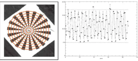
mini-Figure 1. Designated test pattern Siemens star (left), radial modulation analysis for one circle (right) (Reulke et al., 2004).

mum distance between two point sources in order to be resolved by an imaging system. To reduce the subjective influence with bar charts during the determination process some approaches use signal processing techniques to calculate the effective image reso-lution. The method described by Reulke et al. (2004, 2006) is one of the latter approaches. There, the modulation transfer function (MTF) and subsequently the point spread function (PSF) are cal-culated for images with a designated test pattern (e.g. Siemens star). According to the above mentioned approaches the small-est recognizable detail or “the resolution limit is reached if the distance between two points leads to a certain contrast in image intensity between the two maxima.” Using a priori knowledge of the original scene (well-known Siemens star target) the MTF and PSF are approximated by a Gaussian shape function.

M T F=H˜(k)

where MTF (eq. 1) is the modulus of the OTF (optical transfer function) which is equivalent to the PSF in frequency domain (Reulke et al., 2006) and H is the space invariant 2D-PSF (eq. 2), see Figure 1. There are several criteria for the resolving power of cameras. The parameterσ(standard deviation) of the PSF (a Gaussian shape) is one criterion. It directly relates to the image space and can be seen as objective measure to compare different camera performances. Another criterion is the spatial frequency where the MTF reaches a certain (minimal-) value (i.e. 10%, MTF10). The reciprocal of this frequency is the approximation for the number of the smallest line per pixel. The width of PSF at half the height of the maximum is another criterion (full width half maximum - FWHM).

4. DEMOSAICING METHODS

Figure 2. Example of different debayering algorithms.

There is a huge variety of demosaicing algorithms out of we chose several methods (Figure 2) that are widespread and assum-ingly popular.

4.1 Bilinear interpolation

The simplest way to restore the missing information is to inter-polate each channel separately using neighbouring values. Bilin-earinterpolation is the most commonly used mode, but it would be possible to usenearest neighbourorbicubic interpolation in-stead. This method is efficient and straight forward to implement, but images will exhibit colour fringing at edges.

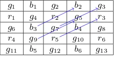
4.2 Variable Number of Gradients (VNG)

VNG reduces colour fringing by using edge detection (Chang et al., 1999). A set of 8 gradients is calculated for each pixel by comparing values in the 5x5 neighbourhood. The gradient is cal-culated by summing up the absolute difference of like-coloured pixels.

g1 b1 g2 b2 g3

r1 g4 r2 g5 r3

g6 b3 g7 b4 g8

r4 g9 r5 g10 r6

g11 b5 g12 b6 g13

Figure 3. Example of gradient calculation forg7according to

Equation 4

The gradient NE (one of eight) at positiong7is calculated by the

following equation:

|g5−g9|+|g3−g7|+|b2−b3|+|r3−r5| (4)

A threshold is used to determine if the pixel lies on a smooth area and averaging can be used to approximate the missing values, or if the pixel lies on a steep gradient, where it is better to use one of two neighbouring values.

4.3 Adaptive Homogeneity-Directed demosaicing (AHD)

Hirakawa and Parks (2005) identify three different classes of arte-facts: misguidance colour artefacts, interpolation colour artefacts and aliasing. They set out to minimize aliasing by using filterbank techniques. Misguidance colour artefacts, which arise when the

Figure 4. Artefact of the AHD algorithm. The maze-like structure on the right is an effect of the algorithm alternating between horizontal and vertical interpolation (G´o´zd´z, 2009).

direction of interpolation is erroneously selected (interpolation along an object boundary is preferable to interpolation across the boundary), are addressed through a nonlinear iterative process. The image is interpolated twice - once verticallyfhand once

hor-izontallyfv. The final outputfis calculated by combingfhand

fvbased on a homogeneity matrixHf which aims to minimize

colour artefacts.

AHD can create visually pleasing images, but there are cases, where it gets confused between vertically or horizontally repeat-ing patterns close to the Nyquist frequency. (see Figure 4).

4.4 MHC (Malvar, He, Cutler)

MHC is a simpler algorithm than VNG or AHD, it has higher performance than such nonlinear algorithms and doesn’t suffer from artefacts due to (sometimes wrong) assumptions about gra-dients in the image (Malvar et al., 2004). It works linearly in a 5x5 neighbourhood by first filling in values using bilinear interpo-lation. It tries to analyse local luminance changes by comparing the actual value at the current pixel position to the value arrived at by interpolating same-colour neighbours. It then factors a corre-sponding gain term when calculating the other two colour values at the same position.

4.5 DCB by Jacek G´o´zd´z

Finally, the iterative DCB algorithm is included. It is largely un-documented, but an open source implementation which performs well is available. (G´o´zd´z, 2009).

4.6 Adobe Camera Raw (as shot)

Adobe Camera Raw is a toolbox in terms of raw image converter and supports a huge variety of image file formats and more portant many camera systems. Although it is a black box im-plementation it yields good results in past investigations but is largely undocumented. However Schewe and Fraser (2010) de-scribe the method according to the selection parameter ‘As Shot’ as follows: “When you select As Shot you allow Camera Raw to attempt to decode the white balance data stored when your cam-era captured the image. Camcam-era Raw may not exactly match the camera’s numbers or its rendering of that white balance, but it does a pretty good job of accessing most cameras’ white balance metadata.”

4.7 Adobe Camera Raw (automatic)

Figure 5. Comparison of different demosaicing methods in terms of (effective) image resolution / resolving power (PSF in pixel).

4.8 Notes

So far, several different demosaicing algorithms have been intro-duced, varying in complexity and performance. It is easy to see that there is no fit-all solution for all scenarios. The method of choice will depend on processing power, whether results should be visually pleasing or geometrically correct, or other factors such as camera lens design since the resulting PSF affects the cor-relation between channels and thus how much information about one channel can be gleaned by analysing another. A further ob-servation is that poorly calibrated white balance can lead to neg-ative visual artefacts with the edge detecting algorithms for the same reason.

The influence of different demosaicing methods regarding resolv-ing power of a camera system suited for UAV applications has been pointed out in (Kraft et al., 2016a). Figure 5 shows the pa-rameterσof the PSF (see section 3) for a Ricoh GXR MountA12 with Zeiss Biogon 21/2.8 lens as a representative of thebridge camera family. The images have been acquired under laboratory conditions. It can be seen that the values forσof PSF change due to the use of different demosaicing methods. While the bilinear approach performs worse in other cases the differences are rather small. Adobe’s Camera Raw (closed source) automatic technique performs best.

During the evaluation process the DCB method provided promis-ing and nearly top-rated results. Additionally and in contrast to Adobes Photoshop Camera Raw Suite it is an open source imple-mentation instead of a black box impleimple-mentation. Therefore we used this demosaicing approach during the experiment / bench-mark (see below).

5. EMPIRICAL UAV CAMERA RESOLUTION TESTS

Having introduced the underlying theory of resolution testing and demosaicing different camera systems will be empirically tested. By this time there is a growing variety of camera systems that either claim to be suited for UAV applications or could be con-sidered suitable because of their specifications (e.g. in terms of sensor size, trigger event control, overall weight, interface ac-cessibility and acquisition costs). These systems are often being grouped as a) systems specifically designed for UAV purposes b) large format cameras, c) system (or bridge-) cameras and d) single-lens reflex cameras. The camera systems compared in this paper are given in Table 1 where Sigma’s DP1 is listed in the categoryOther. The decision was made due to the fact that this

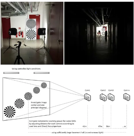
Figure 6. Controlled light conditions (top left), no extraneous light (top right). Illustration of the experiment setup (bottom)

camera has a Foveon-sensor (Hubel et al., 2004) where each pixel element detects colour information instead interpolating neigh-bourhood pixel of a Bayer-pattern arrangement.

5.1 Benchmark layout

The experiment that could (arguably) be appropriate for a bench-mark is motivated and arranged as follows.

Aim is to determine and compare spatial resolution for different sensor-lens combinations. In order to guarantee repeatable mea-surements with identical controlled light conditions and to pre-vent extraneous light a sufficiently large basement hall has been identified (see Figure 6 top). For every camera system the related distance to the designated test pattern (see Figure 6 bottom) has been calculated to ensure identical nominal ground sampling dis-tance (GSD - according to focal length and pixel size on sensor). The GSD in this benchmark has been set to 5mm to address the aforementioned fields of application (e.g. inspection / monitor-ing) including their resolution requirements. Usually, resolving power is changing across the field of view. In order to analyse this effect multiple images have been taken to have the resolution target imaged at different locations in image space (e.g. image center – image half field – image corner). All images have been converted from their raw format to usable tiff format using the same demosaicing algorithm. In this case we chose the DCB method (see Sub-section 4.5) with its open source (C++) imple-mentation of<libraw>and the primordially implementation for DLRs MACS Micro versions<mipps>. For every converted im-age the PSF and correspondingσ(see section 3) has been calcu-lated. To depict the optics resolving power along the sensor di-agonal the ambient noise level (DSNU) and the vignetting effects (PRNU) have not been corrected (see section 2). This should guarantee the genuine system response from object space to sen-sor. The results are presented in Figure 7.

5.2 Discussion

deteriora-Table 1. Specifications of the compared camera systems (* SigmaDP1’s Foveon-chip withtrue4.7Mpx has no Bayer-pattern, therefore no demosaicing necessary)

Average 4,27 3,37

Table 2. Total mean error [cm] for two different UAV camera systems under various block configurations

tion of resolving power is caused by radially symmetric lens dis-tortion and vignetting- effects as clearly can be seen looking at the trend of Sony’s Alpha 7R (with Voigtl¨ander Skopar 35/2.5 lens). Whilst the resolving power in center area is close to top-rated systems it deteriorates extraordinarily to image border.

Imaging performance of all DJI systems is fairly homogenous and the variation in resolving power in comparison to the afore-mentioned sensor-optic combination is quite low. The MACS Micro prototype system (especially the 16 megapixel version) shows top-rated results which (possibly) indicates a connection between pixel size (photon effective area) and resolving power since this sensors pixel pitch is the largest (7.4µm) compared to other systems with Bayer-pattern. The results for resolving power of Sigma’s DP1 support the assumption since its pixel pitch is the most largest (7.8µm). Furthermore the Foveon-chip outperforms all other systems. This could be due to the Bayer-pattern and necessary demosaicing.

Ricoh’s GXR offers a consistent performance and is close to the MACS Micro (12MP) and Phase One’s IXU 1000. Especially the image center resolves close to top-rated value.

The Phase One IXU 1000 with its large sensor format and 100 megapixels shows very low variation in resolving power over the complete image space although it is slightly behind in terms of overall resolution power compared to MACS Micro. Canon’s EOS 5DS R as a representative of the DSLR group is equal to PhaseOne’s IXU but its resolving power diminishes perceptively along the image diagonal.

As it can be seen the blue channel occasionally is determined sig-nificantly worse compared to green channel and especially red channel. The Bayer-pattern arrangement consists of twice the number of pixel for green compared to red respectively blue. Therefore one would expect slightly better results for the green channel but almost equal results for red and blue. This issue is not finally solved and will be investigated in future work considering the presumptions if this problem is either caused by chromatic aberrations and / or colour temperature of the used light source.

Hereafter the results given in this paper are connected to the work of Cramer et al. (2017a). As part of their investigation different UAV camera systems have been calibrated with airborne image data in a calibration field.

Additionally, the influence of different image block configura-tions on the quality of in-situ calibration has been derived for DJI’s Inspire and DJI’s Phantom 3. The obtained quality mea-sures are derived from 22 control points and 23 check points, re-spectively. Only some of the tested block configurations are cited here (see Table 2).

There, the total (mean) error considering all block configurations of the Phantom system (3,37cm) is slightly but significantly better than the Inspire system (4,27cm). The evaluation of radiometric

6. CONCLUSION AND OUTLOOK

The importance of (effective) resolving power as an additional quality measure regarding high resolution requirements for UAV applications has been emphasized and investigated in this pub-lication. A benchmark procedure has been introduced to obtain and evaluate this measure.

A further question is if and how it is possible to determine the impact of radiometrical characteristics on quality of the sub-sequent photogrammetric workflows (e.g. bundle adjustment, Semi-global matching). It is expected that images corrected from falsified values using DSNU and PRNU are more qualified for feature extraction than uncorrected images. Minimized sensor noise (DSNU) and corrected vignetting effects (PRNU) should provide more consistent features especially in outer image re-gions.

Another topic is a) to combine the experiment results under static / laboratory conditions with radiometrical correction parameters (PRNU / DSNU) to provide more fundamental information and b) to verify radiometrical and geometrical quality characteristics presented by Cramer et al. (2017a) under dynamic / operating conditions.

Yet another (technological) field of investigation is the influence of backside illuminated sensors compared with frontside illumi-nated sensor elements.

References

Born, M. and Wolf, E., 1999. Principles of Optics. Cambridge University Press.

Chang, E., Cheung, S. and Pan, D., 1999. Color filter array re-covery using a threshold-based variable number of gradients. Sensors, Cameras, and Applications for Digital Photography.

Cramer, M., Przybilla, H.-J. and Zurhorst, A., 2017a. UAV Cam-eras: Overview and geometric calibration benchmark. submit-ted to this UAV-g 2017 conference, Bonn, Germany.

Cramer, M., Przybilla, H.-J., Meißner, H. and Stebner, K., 2017b. Kalibrierung und Qualit¨atsuntersuchungen UAV-basierter Kamerasysteme.DVW Band 86pp. 67–84.

G´o´zd´z, J., 2009. DCB demosaicing.

http://www.linuxphoto.org/html/dcb.html (April 2016).

Hirakawa, K. and Parks, T. W., 2005. Adaptive homogeneity-directed demosaicing algorithm.IEEE Transactions on Image Processing14(3), pp. 360–369.

Hubel, P. M., Liu, J. and Guttosch, R. J., 2004. Spatial frequency response of color image sensors: Bayer color filters and foveon x3. In:Proc. SPIE, Vol. 5301, pp. 402–407.

Kraft, T., Geßner, M., Meißner, H., Przybilla, H.-J. and Gerke, M., 2016b. Introduction of a photogrammetric camera system for rpas with highly accurate gnss/imu information for stan-dardized workflows. In: J. Skaloud and I. Colomina (eds), EuroCOW 2016, the European Calibration and Orientation Workshop (Volume XL-3/W4), pp. 71–75.

Malvar, H. S., He, L.-w. and Cutler, R., 2004. High-quality linear interpolation for demosaicing of bayer-patterned color images. In:Acoustics, Speech, and Signal Processing, 2004. Proceed-ings.(ICASSP’04). IEEE International Conference on, Vol. 3, IEEE, pp. iii–485.

Mix, P. E., 2005.Introduction to Nondestructive Testing: A Train-ing Guide. JOHN WILEY & SONS INC.

Reulke, R., Becker, S., Haala, N. and Tempelmann, U., 2006. De-termination and improvement of spatial resolution of the CCD-line-scanner system ADS40.ISPRS Journal of Photogramme-try and Remote Sensing60(2), pp. 81–90.

Reulke, R., Tempelmann, U., Stallmann, D., Cramer, M. and Haala, N., 2004. Improvement of spatial resolution with stag-gered arrays as used in the airborne optical sensor ADS40. In: Proceedings of the XXth ISPRS Congress.