GEOREFERENCE OF TERRASAR-X IMAGES
USING NETWORKS OF GROUND CONTROL LINEAR FEATURES
D. I. Vassilakia *
, C. Ioannidisa
, A. A. Stamos b
a
School of Rural and Surveying Engineering,
bSchool of Civil Engineering
National Technical University of Athens, 9 Iroon Polytechniou Str, 15780 Zografos, Greece –
[email protected], [email protected], [email protected]
Commission I, WG I/4
KEY WORDS: Georeferencing, Matching, Feature, SAR, Radar
ABSTRACT:
One of the main novelties introduced by the contemporary spaceborne SAR sensors is the fine Ground Sample Distance (GSD). The GSD of 1 m, which is available now, is comparable to the resolution offered by optical sensors. It creates the conditions to bring closer SAR and optical data and directs research towards SAR processing methods of comparable accuracy with optical processing methods. This paper focuses on the capability offered by contemporary SAR sensors to identify fine man-made and physical features of earth's surface. 3D road edges are treated as Ground Control Information, in order to compute the projective transformation that relates the 3D features of the object space with their 2D projection in a SAR image. The computation of the projection is done with a novel ICP-based method that matches a network of 3D Free-form Linear Features of the object space with their 2D projections in the image space. The proposed method is tested for the georeference of a whole TerraSAR-X scene. Computed results are evaluated with independent Check Points. The quality of the results are superior to those computed with salient point based approaches.
1. INTRODUCTION
SAR is an all-weather, day and night sensor, offering information about the properties of the targets, their 3D geometry and their evolution through time. Contemporary satellite SAR sensors are of high resolution, offering Ground Sampling Distance (GSD) as small as 1 meter. This novel characteristic, makes it possible to identify fine linear characteristics of earth's surface, such as roads (Eineder et al, 2009), which were not possible to identify in data sets collected by the previous generation of satellite SAR sensors. Despite the unprecedented high resolution of contemporary satellite SAR sensors, the identification of salient characteristic points remains an ambiguous process, due to the speckled and fuzzy nature of SAR images, the severe distortions inherited from their geometry and the absence of true color.
This paper takes advantage of the fine resolution introduced by contemporary high resolution SAR sensors, in order to determine a rigorous mathematical relationship between SAR data and heterogeneous (multimodal and multitemporal) remote sensing and geospatial data. Linear features, which are potentially identified more robustly than salient points, are investigated as complementary or even alternative ground control information to salient points, for geometric processes such as georeference and registration.
A novel method based on Iterative Closest Point (ICP) algorithm (Besl and McKay, 1992; Zhang, 1994) is used for accurate and robust heterogeneous free-form linear features (FFLFs) global matching. The method was initially introduced in (Vassilaki et al, 2008a) and (Vassilaki et al, 2008c), in order to match 2D heterogeneous FFLFs with a rigid transformation. It was further expanded in (Vassilaki et al, 2008b), (Vassilaki
et al, 2009b), (Vassilaki et al, 2010b), in order to match FFLFs
of different dimensionality (2D-3D) with non-rigid projective transformation. It does accurate global matching of a single pair of FFLFs of the same (2D-2D, 3D-3D) or of different dimensionality (3D-2D), without constraints on the transformation type, the projection type or the geometric type of the FFLFs. No prior knowledge of points correspondences or FFLFs relative position is required.
In this paper the method is extended and reformed in order to match multiple 3D FFLFs (network) with their 2D projections. The use of networks of FFLFs is required because a single pair of FFLFs may not represent the datasets in their entirety, as it may be confined to a small region of the datasets. The use of multiple pairs of FFLFs also increases the robustness of the whole process. The method is used to recover the relationship between the 3 dimensional object space and its projection in a 2 dimensional TerraSAR-X image. The performance of the proposed method is tested by the georeference of the whole scene of a Single Look Slant Range Complex (SSC) TerraSAR-X image, captured with the High Resolution SpotLight (HS) acquisition mode. The results are compared to those computed through a salient points-based approach.
2. MATCHING NETWORKS OF FFLFs
2.1 The Problem of Matching Networks of FFLFs
In the case of matching networks of FFLFs two unique problems, which are not present in single pair FFLFs matching, have to be faced:
(a) It is generally not known which 3D FFLF corresponds to which 2D FFLF. Thus the correspondences of the FFLFs must be established before application of the ICP
algorithm.
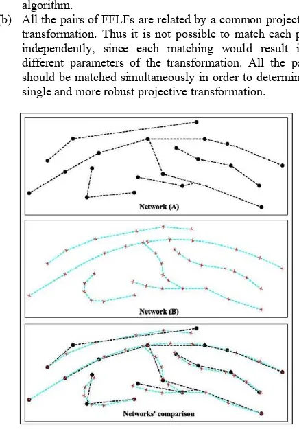
(b) All the pairs of FFLFs are related by a common projective transformation. Thus it is not possible to match each pair independently, since each matching would result into different parameters of the transformation. All the pairs should be matched simultaneously in order to determine a single and more robust projective transformation.
Figure 1. Networks of heterogeneous FFLFs.
2.2 Automated Identification of Correspondent FFLFs
In order to identify the FFLFs correspondences, it is assumed that the two datasets are initially pre-aligned. With this assumption the correspondences would seem easy to identify. A FFLF of the first dataset corresponds to the FFLF of the other dataset which is “closest” to it. However, the definition of “closest” is ambiguous for a FFLF which may span many other FFLFs (Figure 1). Different nodes of the same FFLF may be closest to nodes of different FFLFs. Vassilaki et al, 2009a introduced the term “distance” as a measurement of how far or how different are two FFLFs as a whole. The pair of FFLFs who have the least “distance”, are assumed to correspond to each other. Four candidates for the “distance” were suggested; the euclidean distance between characteristic homologous points such as the first node (d1), the last node (dN), or the centroid (d), and the absolute difference of the FFLFs lengths (ΔS). For robustness, the biggest of these four values can be used as the “distance” of the FFLFs. In the very unlikely case that the “distance” is ambiguous (almost the same) for two or more pairs of FFLFs, application of the full ICP (Vassilaki et al, 2008a) can be used to determine which FFLFs are homologous. ICP is the best and more robust approach, but it is very time consuming and should be avoided if possible.
Manual pre-alignment of the FFLFs is difficult as the varying Z coordinate of the 3D FFLFs and the distortions of the 2D FFLFs due to the SAR sensor make their shapes incompatible. Move, scale and rotate operations are not enough to cancel the non-rigid nature of the SAR projection. Instead, the 3D FFLFs must be projected to the image space of the 2D FFLFs using a good approximation of the unknown projective transformation, which is obtained automatically by a single pair of FFLFs as described in (Vassilaki et al, 2010b). The correspondence of the
single pair of FFLFs is chosen manually by the user, so that in this sense the datasets are manually pre-aligned. However, other than this, the procedure is fully automated.
2.3 Unified One-Step Least Squares Adjustment
The projective transformation is common to all pairs of FFLFs. In order to compute the common transformation the LSM is applied to all the pairs of FFLFs simultaneously. The equations produced by the homologous points of all pairs of FFLFs are assembled into the same LSM matrices. The LSM computes the transformation which best fits all the pairs of FFLFs. The computed transformation brings the FFLFs closer together, and thus the correspondences are reevaluated, in case the previous, poorer, transformation led to a few false correspondences. Each computed pair of closest points, introduces 2 equations, while the unknowns of the problem are the N parameters of the transformation (eg. N=11 for the 3D-DLT projection). Assuming Mi closest points on the ith pair of FFLFs, and m FFLFs, the dimensions of the design matrix [A] of the LSM are:
(
2∑
i=1
m
Mi
)
×N (1)2.4 Matching FFLFs of Different Dimensionality (2D-3D)
The different dimensionality of the FFLFs (3D-2D) is handled through the method proposed in (Vassilaki et al, 2008b; 2009b). The 3D nodes of the 3D FFLFs are projected to the 2D image space using a previous approximation of the projective transformation parameters; the association of each 3D node and its 2D projection is saved. For each 2D node of the projected FFLFs, its closest point in the 2D FFLF is computed, producing 2D-2D pairs. The 2D-2D pairs are converted to 3D-2D pairs through the saved associations. The LSM is applied to the 3D-2D pairs to compute better approximation of the projective transformation parameters.
The steps of the matching algorithm are summarized below: a. Use a single pair of FFLFs to compute the first
approximation of the projective transformation parameters.
b. Project the 3D FFLFs to the image space using the transformation parameters. Save associations of 3D nodes and their projections.
c. Determine FFLFs correspondence by least “distance”. d. For each FFLF pair apply ICP to find 2D-2D pairs of
closest points.
e. Use the association to convert 2D-2D pairs to 3D-2D pairs.
f. Apply LSM to 3D-2D pairs to compute better approximation of the transformation parameters. g. Repeat b-f steps until convergence.
The final result of the algorithm are the matched FFLFs and the projective transformation parameters. The transformation relates the 3D FFLFs, or the object space, to the 2D FFLFs which lie on the image. Because the network of FFLFs spans the image, the transformation in effect relates the image to the object space.
3. APPLICATION
3.1 Test site – Data sets
convenience and usability. The applicability, the efficiency and the accuracy of the method was tested using real data. The study area is in the greater north-eastern region of Athens, Greece. It has steep mountainous terrain, with average elevation 270m and it is generally covered by sparse vegetation. It also includes two small urban regions. The data used are:
(a) a whole scene of a Single Look Slant Range (SSC) TerraSAR-X product which was captured in 2009 with 300 MHz High Resolution SpotLight imaging mode. The scene covers an area of about 50 Km2 (5x10 Km).
(b) a medium scale old topographic map; the original map was in analogue form at a scale of 1:5,000 and it was compiled by stereo-restitution of aerial photos, taken in 1970 (40 years before the acquisition of the satellite image). The map is part of a series which cover the whole territory of Greece. They are readily available for the test and they cost much less than a GPS survey.
The area under study changed widely during the 40 years between the two data collection phases (2009 and 1970). The area used to be an agricultural area but now it exhibits a great variety of land uses, as it serves as a near Athens holiday resort. As in virtually all multitemporal cases, the available map and the image share few common features. Most of these common features are roads which unfortunately evolved through time. Many sections of the roads present wide temporal changes during the 40 years between data acquisitions, as it is shown in the next paragraphs.
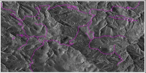
Figure 2. The 2D road network (FFLFs) on the TerraSAR-X image.
Figure 3. The 3D road network (GCLFs) on the old map.
3.2 FFLFs extraction
The 2D road edges extraction was done manually, by digitizing the lines appeared on the data. Most of the roads digitized are paved, as they appear better in the SAR images (Eineder et al,
2009). The road centerlines were obtained from the edges using skeletonization techniques. The road centerline is preferred to road edges as control FFLF, because it has less error than the edges and it fully represents the geometry of the road. The length of the road centerlines varies from a few hundred meters to 8.5 Km (Figures 2 and 3). The contour lines of the map were also digitized. Then they were converted to Triangulated Irregular Network (TIN) via Delaunay triangulation, which was used as DTM in order to extract elevation information of the road centerlines. The road centerline profiles are in general rough, due to the scale of the map and the fact that the map does not have elevation information along the surface of the road. The centerline elevation was computed by the surrounding terrain.
3.3 Mathematical Model
Four distinct projection models were used to test the method; first and second order 3D Polynomial Functions (PFs) (Toutin, 2004), 3D Direct Linear Transform (DLT) and 3D Rational Polynomial Functions (RPFs) of first order, with 8, 16, 11 and 14 unknown parameters respectively (Eq. 2 to 5).
x=a1Xa2Ya3Za4 y=b1Xb2Yb3Zb4 (2) applied to real data in a high relief area with a variety of land-uses (urban, agricultural and forest land), in order to investigate the performance of the method.
3.4 Tests and Results
Three different cases were tested. For all the tests, a preliminary georeference was computed using a single pair of correspondent FFLFs. The computed projective transformation was used to bring the FFLFs close together.
In the first test (Test A) the centerlines of 4 roads were used as Ground Control Linear Features (GCLFs). Using the preliminary georeference it was possible to determine and eliminate the sections of the roads which exhibited wide temporal changes.
In the second test (B) the centerlines of 14 roads were used as GCLFs. In this test the whole lengths of the roads were used, regardless of the temporal changes that were identified.
In the third test (C) the same 14 centerlines as in (B) were used, but the sections of the roads which exhibited wide temporal changes were eliminated as identified in (B).
Figure 4. Test A: Matching results.
Figure 5. Test B: Matching results.
Figure 6. Test C: Matching results.
Figure 7. Test B: Road sections with wide temporal changes.
In order to check the accuracy of the georeference, 16 independent Check Points (CPs), which were extracted from the medium scale old map and were identified in the SAR image were used. Figure 8 shows the distribution of the CPs.
Figure 8. CPs distribution.
Table 1 shows the RMSE (in pixels) computed by the 16 CPs using the 4 projective transformation models (first and second order PFs, DLT and RPFs), for each one of the 3 tests (A, B and C). In addition, Table 2 and Figure 9 show the residual of each CP using the 4 models, for test C.
Test 1
st order PF 2nd order PF DLT RPF
dRg dAz dRg dAz dRg dAz dRg dAz
A 4.7 4.5 4.9 4.7 4.1 4.7 4.4 3.9
B 4.2 3.9 5.3 4.7 5.7 4.2 5.0 5.2
C 4.1 3.6 4.8 3.7 4.2 3.7 4.4 3.8
Table 1. CPs RMSE (pixels), in Range and Azimuth.
CP 1 st
order PF 2nd
order PF DLT RPFs
dRg dAz dRg dAz dRg dAz dRg dAz
1 5.9 5.6 7.4 6.0 5.1 5.2 3.7 5.5
Table 2. Test C: Residuals and RMSE (pixels) of CPs.
3.5 Evaluation of the Results
The RMSE is almost the same regardless the projective transformation used (Figure 9, Tables 1 & 2). The differences (1.5 pixel at most), are statistically insignificant as they are less than the accuracy of the map (approximately 3 pixels). Furthermore, the uncertainty of the point location on the SAR image is larger than 1 pixel. In the first test (A) the GCLFs are only 4, but they cover adequately the scene. In the second test (B) the GCLFs contain gross error in various sections with higher order does not imply higher accuracy if the underlying problem does not have this accuracy (Press et al, 1992) as it is in the present case.
The tests show that the method is insensitive to temporal changes, given the abundance of GCLFs found in all types of data. The method manages to match robustly and efficiently data which contain sections with gross temporal changes, producing low RMSE. The method can also be used to identify these segments and exclude them from the matching.
The results are of superior quality to those computed by salient point based approaches. In (Vassilaki and Ioannidis, 2010) a terrain dependent approach was used in order to georeference a High Resolution SpotLight TerraSAR-X image, using the DLT (11 parameters) and the 1st order RPF (14 parameters). The RMSE of independent CPs were about 4-7 pixels in range and about 3.5-5 in azimuth direction. About the same results were later computed by (Crespi et al, 2010), who used a terrain independent approach to georeference a SpotLight CosmoSkyMed image, using 3rd order RPFs (78 parameters, 20 of which proved to be statisticalllysignificant). In (Nonaka et al, 2008) a digital map at a scale of 1:2500 was used in order to evaluate the accuracy of the orthorectified EEC SpotLight TerraSAR-X products. The accuracy revealed to be better than 5 m in a flat area while it degraded to more than 10 m in mountainous areas.
4. CONCLUSIONS
In this paper a new method for the georeference of TerraSAR-X images was presented. The method computes the projective transformation model between the 3D object space and its 2D projection in the image, using GCLFs instead of the traditionally used GCPs. The performance of the method was tested by the georeference of the whole scene of a Single Look Slant Range Complex (SSC) TerraSAR-X image, captured with the High Resolution SpotLight (HS) acquisition mode. The accuracy of the proposed method was tested with independent CPs. The RMSE of the CPs was about 4 pixels in the GCLFs leaves little doubt about the reliability of ground control information (GCI), as compared to the often ambiguous and (NSRF) - Research Funding Program: Heracleitus II. Investing in knowledge society through the European Social Fund. The authors are also grateful to the SRSE of NTUA for providing the SAR data and prof. V. Pagounis and students of TEI-A for the digitization of the maps.
REFERENCES
Besl, P.J. and McKay, N.D., 1992. A Method for Registration of 3-D Shapes. IEEE Transactions on Pattern Analysis and Machine Intelligence, 14(2), pp. 239-256.
Crespi, M., Capaldo, P., Fratarcangeli, F., Nascetti, A., Pieralice, F., 2010. DSM generation from very high optical and radar sensors: Problems and potentialities along the road from the 3D geometric modeling to the surface model. IEEE International Geoscience and Remote Sensing Symposium, pp. 3596-3599.
Eineder, M., Adam, N., Bamler, R., Yaque-Martinez, N., Breit, H., 2009. Spaceborne Spotlight SAR Interferometry with TerraSAR-X. IEEE Transactions on Geoscience and Remote Sensing, 47(5), pp. 1524-1535.
Stamos, A.A., 2007. ThanCad: a 2dimensional CAD for engineers. Proceedings of the Europython2007 Conference,
Vilnius, Lithuania.
Toutin, Th., 2004. Review Paper: Geometric processing of remote sensing images: models, algorithms and methods,
International Journal of Remote Sensing, 25(10), pp. 1893-1924.
Vassilaki, D.I, Ioannidis, C. and Stamos, A.A., 2008a. Registration of 2D Free-Form Curves Extracted from High Resolution Imagery using Iterative Closest Point Algorithm.
EARSeL's Workshop on Remote Sensing – New Challenges of High Resolution, March 5-7, Bochum, Germany, pp.141-152.
Vassilaki, D.I., Ioannidis, C., Stamos, A.A., 2008b. Computation of the Closest Points for Matching Curves of Different Dimensionality. 3rd International Conference: From Scientific Computing to Computational Engineering, July 9-12, Athens, Greece (on CD-ROM).
Vassilaki, D.I., Ioannidis, C. and Stamos, A.A., 2008c. Geospatial Data Integration using Automatic Global Matching of Free-Form Curves. Digital Earth Summit on Geoinformatics 2008: Tools for Global Change Research, Wichmann Verlag, Heidelberg, pp. 195-200.
Vassilaki, D.I., Ioannidis, C. and Stamos, A.A., 2009a. Multitemporal Data Registration through Global Matching of Networks of Free-form Curves. FIG Working: Surveyors Key Role in Accelerated Development, May 3-8, Eilat, Israel.
Vassilaki, D.I., Ioannidis, C. and Stamos, A.A., 2009b. Registration of Unrectified Optical and SAR imagery over Mountainous Areas through Automatic Free-form Features Global Matching. International Archives of Photogrammetry, Remote Sensing and Spatial Information Sciences, (38), Part 1-4-7/W5 (on CD-ROM).
Vassilaki, D.I. and Ioannidis C., 2010a. Georeference of High Resolution TerraSAR-X Images with RPFs. 30th EARSeL Symposium: Remote Sensing for Science, Education, and Natural and Cultural Heritage, pp. 573-580.
Vassilaki, D.I., Ioannidis, C. and Stamos, A.A., 2010b. Enhanced First Approximation for ICP-based Global Matching of Free-form Curves in Side-looking Radar Geometry.
International Archives of Photogrammetry, Remote Sensing and Spatial Information Sciences, (38), Part 3A, pp. 85-90.