THE EFFECTS OF LASER REFLECTION ANGLE ON RADIOMETRIC CORRECTION
OF THE AIRBORNE LIDAR INTENSITY DATA
Ahmed Shaker*, Wai Yeung Yan, Nagwa El-Ashmawy
Department of Civil Engineering, Ryerson University, Toronto, Ontario, Canada - (ahmed.shaker, waiyeung.yan, nagwa.elashmawy)@ryerson.ca
KEY WORDS: Radiometric Correction, LiDAR, Intensity Data, Reflection Angle, Surface Normal, Land Cover Classification
ABSTRACT:
Radiometric correction (RC) of the airborne Light Detection And Ranging (LiDAR) intensity data has been studied in the last few years. The physical model of the RC relies on the use of the laser range equation to convert the intensity values into the spectral reflectance of the reflected objects. A number of recent studies investigated the effects of the LiDAR system parameters (i.e. range, incidence angle, beam divergence, aperture size, automatic gain control, etc.) on the results of the RC process. Nevertheless, the condition of the object surface (slope and aspect) plays a crucial role in modelling the recorded intensity data. The variation of the object surface slope and aspect affects the direction as well as the magnitude of the reflected laser pulse which makes significant influence on the bidirectional reflectance distribution function. In this paper, the effects of the angle of reflection, which is the angle between the surface normal and the incidence laser pulse, on the RC results of the airborne LiDAR intensity data is investigated. A practical approach is proposed to compute the angle of reflection using the digital surface model (DSM) derived from the LiDAR data. Then, a comparison between the results of the intensity data after RC using the scan angle and RC using the angle of reflection is carried out. The comparison is done by converting the intensity data into equivalent image data and evaluating the classification results of the intensity image data. Preliminary findings show that: 1) the variance-to-mean ratio of the land cover features are significantly reduced while using the angle of reflection in the RC process; 2) 4% of accuracy improvement can be achieved using the intensity data corrected with the scan angle. The accuracy improvement increases to 8% when using the intensity data corrected with the angle of reflection. The research work practically justifies the use of the reflection angle in the RC process of airborne LiDAR intensity data.
* Corresponding author.
1. INTRODUCTION
The importance of the radiometric correction (RC) of the airborne LiDAR intensity data has been addressed in the last few years (Coren and Sterzia 2006; Höfle and Pfeifer 2007; Wagner, 2010). Similar to all active sensors, the objective of the RC of the LiDAR intensity data is to remove the attenuation of the received laser energy with respect to atmospheric and surface conditions. The results of the RC can be used to derive the spectral reflectance of the reflected energy from objects in the near-infrared red wavelength. High separability amongst different land cover classes can always be found in this spectrum region. The ultimate goal of the RC is to maximize the benefit of using the LiDAR intensity data for a variety of applications in feature extraction and object recognition. Physical approach of RC has been initially proposed by Coren and Sterzia (2006) and Höfle and Pfeifer (2007) based on the use of the laser range equation. The correction model considers the system parameters (sensor dependent) and the environmental parameters (location dependent) in order to convert the recorded intensity data into its corresponding spectral reflectance values. The significance of the RC on the airborne LiDAR intensity data has been proven recently. Korpela et al. (2010) conducted tree classification using discrete-return LiDAR data. 6% to 9% of accuracy improvement is found after the normalization of the range and automatic gain control of the intensity data. Yan et al. (2011) compared different land cover classification scenarios using the airborne LiDAR intensity data in an urban area. Although the
overall accuracy ranges from 30% to 60%, an accuracy improvement is found by 8% to 12% using the radiometrically corrected LiDAR intensity data.
In order to develop an optimal model for RC, the effects of LiDAR system parameters were investigated in a number of research work. The research team from Finnish Geodetic Institute made extensive effort to study the impacts of the system parameters on radiometric calibration such as range (Kaasalainen et al., 2009), incidence angle (Kukko et al., 2008), aperture size (Kaasalainen and Kaasalainen, 2008), flying height (Vain et al., 2009), and the automatic gain control (Vain et al., 2010) by conducting laboratory and field measurements. Practical methods were developed to derive the surface reflectance by eliminating the effects of these parameters through absolute correction and relative calibration approaches. The condition of the object surface slope and aspect plays a crucial role in modelling the recorded intensity data. The variation of the topography (slope and aspect) affects the size of the projected footprint (Sheng, 2008) and the backscattered laser pulse (Kukko et al., 2008) which makes significant influence on the bidirectional reflectance distribution function (BRDF). Therefore, consideration of the surface normal of objects is needed to determine an accurate reflection angle regardless of the reflection models (Jutzi and Gross, 2010). This paper aims to examine the use of the angle of reflection for RC of airborne LiDAR intensity data. Although a number of previous studies addressed the calculation of surface normal from the LiDAR data, most of them are computational intensive.
In this work, we propose a set of equations for computing the angle of reflection based on the digital surface model (DSM) generated from the LiDAR data point cloud. A comparison of the results is presented before and after incorporating the angle of reflection in the RC process. It is hoped that the information presented in this paper will be able to fill part of the information gap in the development of a comprehensive correction model for the airborne LiDAR intensity data.
2. RADIOMETRIC CORRECTION
2.1 Laser Range Equation
The laser range equation (Jelalian, 1992) describes the physical properties of the laser beam energy with respect to the sensor configuration and different environmental parameters. The equation is used to convert the LiDAR intensity data (which is direct proportional to the amount of received laser energy Pr)
where Ptis the transmitted laser pulse energy, Dr is the diameter of the aperture, R is the range, βt is the laser beam width, sys is the system factor, and atm is the atmospheric attenuation factor which is assumed as a constant in some of the previous studies. In this study, we model the atmospheric attenuation as the summation of aerosol scattering, molecular scattering, and molecular absorption based on the Beer-Lambert Law. Details can be found in Yan et al. (2011).
Figure 1. Illustration of the angle of reflection ( r)
The target cross section σ consists of all target characteristics including the spectral reflectance ρ, the projected target area to the direction of the laser beam A, and the direction of reflection which is determined by the angle between the LiDAR sensor and the target. In case of inclined surface, the cosine should be the cosine of the angle of reflection r which is the angle between the surface normal and the incidence laser pulse as illustrated in figure 1. Nevertheless, few of the previous research work emphasize the importance of the computation of the reflection angle in the RC process. Therefore, section 2.2 describes the mathematical procedures to calculate the r.
2.2 Computation of the Angle of Reflection
Figure 2 presents the geometric relationship between the instantaneous position of the LiDAR sensor (L) and the object on the ground (P) in a XYZ Cartesian coordinate system. The scan angle denotes as and the distance between the sensor and the ground object is represented by the range R. In case of flat terrain, the angle of reflection is described between two vectors which are the vertical vector from the ground object (PV
→ as well as the surface normal vector (PN
→
) to the ground object. In this study, the slope (α) and aspect (β) are determined by using the DSM derived from the LiDAR data.
Figure 2. Illustration of the geometric relationship between the LiDAR sensor (L) and the surface of the ground object (P)
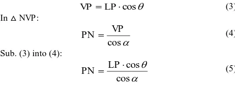
can be calculated from the following equations. In △LVP:
can be calculated from the following equations. In △LVP:
where angle ∠YVN is a reflex angle which is equal to the aspect of the ground object P on the terrain. The angle ∠YVL is equal to the projected horizontal angle between the Y-axis and the laser pulse plus 180°. The projected horizontal angle ∠YVL can be computed using the plane coordinates of the laser pulse and the instantaneous position of the LiDAR sensor derived from the GPS trajectory. According to the cosine law:
NVL
LVNV LV
NV
NL 2 22 cos (10)
Finally, the angle of reflection ∠LPN can be calculated using the three vectors (LP
→ , PN
→
, and LN →
) in the triangle LPN in accordance to the cosine law:
In △LPN:
LP PN
LN LP PN LPN
2 cos
2 2 2 1
(11) where LP
→
is the range vector, PN →
can be obtained in eq. (5), and NL
→
can be obtained in eq. (10).
3. METHODOLOGY
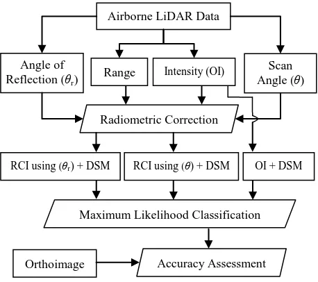
Figure 3 shows the experimental workflow of the research work. The airborne LiDAR data point cloud obtained for the study area (in LAS format) is pre-processed before RC. The range and the scan angle of each of the laser pulse are computed by using the GPS trajectory data and the xyz coordinates of the point cloud. The angle of reflection for each laser pulse is calculated as explained in section 2.2. The scan angle ( ) and the angle of reflection ( r) are imported to the laser range equation (with all the system and environmental parameters discussed in section 2.1) resulting two RC intensity datasets: i) RCI using ( ) and ii) RCI using ( r)).
Figure 3. Experimental workflow
Maximum likelihood classification technique is conducted on the original intensity (OI) and the two RCI datasets together with the DSM individually for land cover classification in order to evaluate the effect from the use of the reflection angle on the corrected intensity data.
Several classification scenarios of different number of land cover classes are conducted on the LiDAR datasets. The classes design follows the standardized national Land Cover Classification Scheme (LCCS) from the United States Geological Survey (USGS) (Anderson et al., 1976). The first scenario classifies the study area into two land cover classes: i) urban or built-up land (Class 1 in Level I of USGS LCCS), and ii) rangeland (Class 3 in Level I of USGS LCCS). The urban or built-up lands mainly consist of roads, parking lots, pavements, and buildings. The rangeland includes mixed grass coverage and trees mostly in the West part of the study area. The second scenario subdivides the rangeland into high rangeland (trees) and low rangeland (grass) creating the three land cover classes: i) urban or built-up land, ii) trees, and iii) grass land. The third scenario further subdivides the rangeland into i) trees, ii) grass land, and iii) barren land (Class 7 in Level I of USGS LCCS). The four classes of the third scenario include the three subdivided rangeland and the urban or built-up land class. The last scenario subdivides the urban or built-up class into roads and buildings (Level II of USGS LCCS). The five land cover classes are: i) roads, ii) buildings, iii) trees, iv) bare soil, and v) grass land. Accuracy assessment is carried out on the classification results by using 1000 checkpoints with reference to the ortho-rectified aerial photo captured during the same flight of LiDAR survey. Overall accuracy of the classification results are computed for the comparative analysis.
4. STUDY AREA
The study area (500 x 400 m) covers the British Columbia Institute of Technology (BCIT) located at the Burnaby, British Columbia, Canada (122°59’W, 49°15’N). A single strip of the airborne LiDAR data captured by Leica ALS 50 sensor is used for the experimental testing. The LiDAR sensor is operated in 1.064 μm wavelength, the beam divergence is 0.33 mrad, and the pulse repetition frequency is 83 kHz. The average flying height is 600 m which leads to a point density of 4 to 5 points per meter square. The direction of the flight survey for this subset of data is from West to East. The reason of selecting this particular area of the BCIT campus is mainly due to the variety of the land cover features with varying elevation. The area contains buildings, parking lots connected by sidewalks and pavements, shrubs and open spaces with grassy coverage. Figure 4 shows the ortho-rectified aerial photo of the study area.
Figure 4. The study area at British Columbia Institute of Technology, B.C., Canada
Airborne LiDAR Data
Radiometric Correction
Scan Angle ( ) Angle of
Reflection ( r)
Maximum Likelihood Classification
Accuracy Assessment Range Intensity (OI)
RCI using ( r) + DSM RCI using ( ) + DSM OI + DSM
Orthoimage
5. RESULTS AND ANALYSIS
5.1 Radiometric Correction
In order to evaluate the effects of the RC and the effects from the use of the reflection angle, the variance-to-mean ratio of the intensity values of different land cover features are computed for: i) OI, ii) RCI using ( ), and iii) RCI using ( r) as shown in Table 1. Generally, a small value of variance-to-mean ratio indicates a small variation of intensity values within a specific land cover feature and it reveals the homogeneity of the intensity values recorded for that land cover feature. Ten targets are selected for each of the land cover feature and the total number of LiDAR data points is approximate 2500 in each land cover feature. It is found that the variance-to-mean ratio of different land cover features is reduced after RC. The reduction of the variance-to-mean ratio ranges from 16% to 32% after RC using depending on the land cover type. The reduction further increases when using the angle of reflection ( r) for the RC process. The variance-to-mean ratio decreased by 88%, 85%, and 75% for the building, road and vegetation samples, respectively. The relatively low reduction of variance-to-mean ratio in vegetation samples can be ascribed by the mixture of different grass and soil samples which lead to the large variation of intensity values. Despite of this, the results show the main benefit from using the reflection angle in the RC process to produce more homogenous intensity values for same features.
Num. of Samples
Original Intensity
RCI using ( )
RCI using ( r)
Building 2,720 4.753 3.992 0.566
Road 2,306 0.849 0.649 0.131
Vegetation 2,447 4.953 3.326 1.231
Table 1. Variance-to-mean ratio of different land cover features before and after radiometric correction.
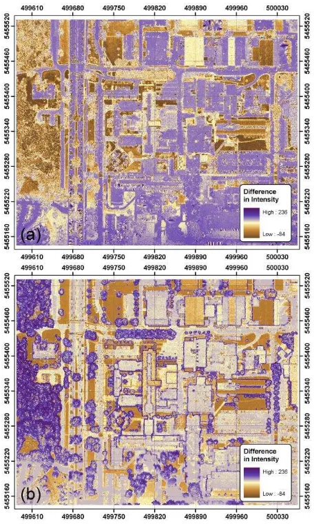
The changes between the OI and RCI data are presented in figure 5, which shows the difference between the OI and the RCI using ( ). The major difference of the intensity values (purple color) can be located at the edge of the study area (North and South area) and at the terrain with low elevation. This is mainly because of the long range and large scan angle which lead to a large RC in accordance to the laser range equation. Elevated features such as buildings and trees receive less correction as they are close to the LiDAR sensor as shown in figure 5(a). Nevertheless, RC using the angle of reflection ( r) gives completely different results for the intensity data. As shown in figure 5(b), large difference of intensity values can be found at the trees and buildings. This can be explained due to the incorporation of the surface normal which leads to a large correction for these features. It is obvious that by using the reflection angle, one can easily distinguish the trees from the grass and soil visually based on intensity values.
Figure 5. The changes in intensity data presented by differences of the digital numbers before and after radiometric correction
using a) scan angle ( ) and b) angle of reflection ( r)
5.2 Land Cover Classification
Table 2 shows the overall accuracy of the four classification scenarios by using the three datasets (OI, RCI using ( ), and RCI using ( r)). DSM is incorporated with the intensity data as an ancillary data for the land cover classification. In general, the overall accuracy of the classification results after RC is always higher than the results from the original intensity data. Comparing the results of both RCI dataset using ( ) and ( r), the overall accuracy of the classification results using the angle of reflection ( r) is always higher than the results using the scan angle ( ).
OI + DSM
RCI ( ) + DSM
RCI ( r) + DSM
2-Classes 75.17% 77.05% 78.85%
3-Classes 67.42% 69.88% 72.24%
4-Classes 60.81% 61.00% 68.65%
5-Classes 40.23% 44.29% 46.27%
Table 2. Overall accuracy of the four land cover classification scenarios
For the 2-classes scenario, the accuracy of the original intensity data with DSM reaches over 75%. The overall accuracy increases by 1.9% and 3.7% by using the RCI with ( ) and RCI with ( r), respectively. Although the overall accuracy of the OI drops to 67% in the 3-classes scenario, improvement of the classification accuracy is still recorded by using both RCI datasets. The classification result of RCI ( r) + DSM has an accuracy improvement of 4.8% whereas the accuracy of classification result using RCI ( ) + DSM improves 2.4%. In the 4-classes scenario, the overall accuracy of the OI+DSM is just over 60%. The RC using the scan angle ( ) does not help in distinguishing the tree, grass, and barren land resulting in less than 1% improvement. With the consideration of the surface normal, the RCI ( r) is useful to provide high separability amongst the three natural covers and thus 8% of accuracy improvement is recorded in the classification result. In the 5-classes scenario, the spectrum mixture of the construction materials in building rooftop and asphalt road causes a significant drop of the classification accuracy by 20%. Despite of that, an accuracy improvement of 4% and 6% is still observed in the classification results using RCI ( ) + DSM and the RCI ( r) + DSM, respectively in the 5-classes scenario. To conclude, 0% to 4% of accuracy improvement is found in the classification results using the RCI using ( ) + DSM. A double of the accuracy improvement (4% to 8%) can be achieved in the classification results using the RCI using ( r) + DSM.
6. CONCLUSIONS
In this study, we propose a practical approach to compute the angle of reflection using the DSM derived from the LiDAR data point cloud. The angle of reflection is imported to the laser range equation together with all the parameters (i.e. range, intensity and atmospheric attenuation factor) to radiometrically correct the airborne LiDAR intensity data. To evaluate the impact of the reflection angle on the RC intensity data, the scan angle is used to carry out the same process. With the incorporation of DSM, the RC intensity datasets and the original intensity data are used to conduct land cover classification individually for different scenarios.
Statistical analysis reveals that the variation of the intensity value is significantly reduced within the same land cover feature after applying the RC. The phenomenon is more obvious in the case of using the angle of reflection for RC in both analyses. For the land cover classification, the overall accuracy ranges from 40% to 75% using the original LiDAR intensity data (OI +DSM). 0% to 4% of accuracy improvement is found in the classification results using the RCI using scan angle ( ) + DSM. A double of the accuracy improvement (4% to 8%) can be achieved in the classification results using the RCI using reflection angle ( r) + DSM. The study practically proves that 1) the angle of reflection should be utilized in the laser range equation instead of the scan angle in the RC process, and 2) RC should be applied on the airborne LiDAR data since it improves the classification accuracy.
7. ACKNOWLEDGEMENTS
This research work is supported by the Discovery Grant from the Natural Sciences and Engineering Research Council of Canada (NSERC) and the GEOIDE Canadian Network of Excellence, Strategic Investment Initiative (SII) project SII P-IV # 72. The authors would like to thank Prof. Ayman Habib
and his research team from the University of Calgary and the McElhanney Consulting Services Ltd., B.C., Canada for providing the real LiDAR and image datasets.
8. REFERENCES
Anderson, J.R., Hardy, E.E., Roach, J.T., and Witmer, R.E. 1976. A land use and land cover classification system for use with remote sensor data. Geological Survey Professional Paper 964. U.S. Geological Survey, Washington, DC. pp. 28.
Coren, F., and Sterzai, P. 2006. Radiometric correction in laser scanning. Int. J. of Remote Sensing, 27 (15), pp. 3097-3014. Höfle, B., and Pfeifer, N. 2007. Correction of laser scanning intensity data: Data and model-driven approaches. ISPRS J. of Photogrammetry & Remote Sensing, 62(6), pp. 415-433. Jelalian, A.V., 1992. Laser Radar Systems. Artech House, Boston, London, 292 pp.
Jutzi, B., and Gross, H. 2010. Investigations on surface reflection models for intensity normalization in airborne laser scanning (ALS) data. Photogrammetric Engineering & Remote Sensing, 76 (9), pp. 1051-1060.
Kaasalainen, M., and Kaasalainen, S. 2008. Aperture size effects on backscatter intensity measurements in Earth and space remote sensing. J. of Optical Society of America A, 25(5), pp. 1142-1146.
Kaasalainen, S., Krooks, A., Kukko, A., and Kaartinen, H. 2009. Radiometric calibration of terrestrial laser scanners with external reference targets. Remote Sensing, 1(3), pp. 144-158. Korpela, I., Ørkab, H.O., Hyyppäc, J., Heikkinen, V., and Tokola, T. 2010. Range and AGC normalization in airborne discrete-return LiDAR intensity data for forest canopies. ISPRS J. of Photogrammetry & Remote Sensing, 65(4), pp. 369-379. Kukko, A., Kaasalainen, S., Litkey, P. 2008. Effect of incidence angle on laser scanner intensity and surface data. Applied Optics, 47 (7), pp. 986-992.
Sheng, Y. 2008. Quantifying the size of a LiDAR footprint: A set of generalized equations. IEEE Geoscience and Remote Sensing Letters, 5(3), pp. 419-422.
Vain, A., Kaasalainen, S., Pyysalo, U., Krooks, A., and Litkey, P. 2009. Use of naturally available reference targets to calibrate airborne laser scanning intensity data. Sensors, 9(4), pp. 2780-2796.
Vain, A., Yu, X., Kaasalainen, S., and Hyyppä, J. 2010. Correcting airborne laser scanning intensity data for automatic gain control effect. IEEE Geoscience and Remote Sensing Letters, 7(3), pp. 511-514.
Wagner, W. 2010. Radiometric calibration of small-footprint full-waveform airborne laser scanner measurements: Basic physical concepts. ISPRS J. of Photogrammetry and Remote Sensing, 65(6), pp. 505-513.
Yan, W.Y., Shaker, A., Habib, A., and Kersting, A. P. 2011. Improving classification accuracy of airborne LiDAR intensity data by geometric calibration and radiometric correction. ISPRS J. of Photogrammetry and Remote Sensing (Submitted)