ANALYZING THE APPLICABILITY OF THE LEAST RISK PATH ALGORITHM IN
INDOOR SPACE
A. Vanclooster a,*, P. Viaenea, N. Van de Weghea, V. Fackb, Ph. De Maeyer a
Ghent University, Krijgslaan 281, B-9000 Ghent, Belgium
a
Dept. of Geography - (Ann.Vanclooster, Pepijn.Viaene, Nico.VandeWeghe, Philippe.DeMaeyer)@UGent.be
b
Dept. of Applied Mathematics and Computer Science - [email protected]
*
Corresponding author
KEY WORDS: Indoor navigation, 3D algorithms, cognitive wayfinding
ABSTRACT:
Over the last couple of years, applications that support navigation and wayfinding in indoor environments have become one of the booming industries. However, the algorithmic support for indoor navigation has so far been left mostly untouched, as most applications mainly rely on adapting Dijkstra’s shortest path algorithm to an indoor network. In outdoor space, several alternative algorithms have been proposed adding a more cognitive notion to the calculated paths and as such adhering to the natural wayfinding behavior (e.g. simplest paths, least risk paths). The need for indoor cognitive algorithms is highlighted by a more challenged navigation and orientation due to the specific indoor structure (e.g. fragmentation, less visibility, confined areas…). Therefore, the aim of this research is to extend those richer cognitive algorithms to three-dimensional indoor environments. More specifically for this paper, we will focus on the application of the least risk path algorithm of Grum (2005) to an indoor space. The algorithm as proposed by Grum (2005) is duplicated and tested in a complex multi-story building. Several analyses compare shortest and least risk paths in indoor and in outdoor space. The results of these analyses indicate that the current outdoor least risk path algorithm does not calculate less risky paths compared to its shortest paths. In some cases, worse routes have been suggested. Adjustments to the original algorithm are proposed to be more aligned to the specific structure of indoor environments. In a later stage, other cognitive algorithms will be implemented and tested in both an indoor and combined indoor-outdoor setting, in an effort to improve the overall user experience during navigation in indoor environments.
1. INTRODUCTION AND PROBLEM STATEMENT
Over the last decade, indoor spaces have become more and more prevalent as research topic within geospatial research environments (Worboys, 2011). Within indoor research, applications that support navigation and wayfinding are of major interest with both technological advancements for tracking people (Mautz et al., 2010) as well as developments of the underlying space frameworks (e.g. Lee, 2004).
However, the algorithmic support for indoor navigation applications has so far been left mostly untouched. In outdoor research, a wide variety of different algorithms exist, initially originating from shortest path algorithms (Cherkassky et al., 1996) with many of them based on the famous Dijkstra shortest path algorithm (Dijkstra, 1959). Over time, alternative algorithms were proposed adding a more cognitive notion to the calculated paths and as such adhering to the natural wayfinding behavior in outdoor environments. Examples are hierarchical paths (Fu et al., 2006), paths minimizing route complexity (Duckham & Kulik, 2003; Richter & Duckham, 2008) or optimizing risks along the described routes (Grum, 2005). The major advantage of those algorithms is their more qualitative description of routes and their changed embedded cost function. After all, various cognitive studies have indicated that the form and complexity of route instructions is equally important as the total length of path (Duckham & Kulik, 2003). Algorithms which simplify the use and understanding of the calculated routes improve as such the entire act of navigation and wayfinding.
Algorithms for 3D indoor navigation are currently restricted to Dijkstra or derived algorithms. To date, only few researchers have attempted to approach algorithms for indoor
navigation differently, for example incorporating dynamic events (Musliman et al., 2008), or modeling evacuation situations (Atila et al., 2013; Vanclooster et al., 2012). However, the need for more cognitively rich algorithms is even more pronounced in indoor spaces than outdoors. This has its origin in the explicit distinctiveness in structure, constraints and usage between indoor and outdoor environments (Li, 2008; Walton & Worboys, 2009). Also, wayfinding tasks in multi-level buildings have proven to be more challenging than outdoors, for reasons of disorientation and less visual aid (Hölscher et al., 2009). As such, building occupants are faced with a deficient perspective on the building structure, influencing their movement behavior (Hölscher et al., 2009). Algorithms developed to support a smooth navigation will have to consider these intricacies and create route instructions that are more aligned with the human cognitive mapping of indoor spaces.
The main goal of this paper is to translate existing outdoor cognitive algorithms to an indoor environment and compare their efficiency and results in terms of correctness, difference to common shortest path algorithms and their equivalents in outdoor space. Based on the results of this implementation, suggestions for a new and improved cognitive algorithm will be stated, which will be more aligned to the specific context of indoor environments and wayfinding strategies of users indoor. In this paper, we currently focus on the implementation and adjustment of the least risk path algorithm (LRP algorithm hereafter) as described by Grum (2005).
The remainder of the paper is organized as follows. Section 2 elaborates on the definition of the LRP algorithm. In section 3, the indoor dataset is presented while section 4 discusses ISPRS Annals of the Photogrammetry, Remote Sensing and Spatial Information Sciences, Volume II-4/W1, 2013
the main case study where the outdoor LRP algorithm is duplicated and implemented in an indoor setting with multiple analyses comparing its results. Section 5 presents various improvements to the original algorithm to be more compatible with indoor networks.
2. LEAST RISK ALGORITHM
The ultimate goal of cognitive algorithms is to lower the cognitive load during wayfinding experiences. In this paper we focus on the LRP algorithm (Grum, 2005) and its implementation in a three-dimensional building. More specifically, we want to investigate whether or not the least risk path has the same connotation and importance in indoor spaces compared to its original outdoor setting.
The LRP algorithm as defined by Grum (2005), calculates the path between two points where a wayfinder has the least risk of getting lost along the path. The risk of getting lost is measured at every intersection with the risk cost calculated as a cost for taking the wrong decision at that intersection. While the algorithm assumes that an unfamiliar user immediately notices a wrong choice and returns to the previous intersection, the author also acknowledges that the algorithm needs to be tested for its representativeness of the actual behavior of users (Grum, 2005).
The formula for the calculation of the risk value at a certain intersection i and the total risk of an entire path p is as follows:
choices possible
choices wrong
length i
Value Risk
_ _ _
* 2 ) (
_ = (1)
+
= risk values i lengths p
Risk
Total_ ( ) _ () (2)
Formula 1 demonstrates that the risk value (RV) is dependent on the number of street segments converging on the intersection, combined with the length of each individual segment. The risk value of an intersection increases with more extensive intersections and with many long edges that could be taken wrongly. The algorithm favors paths with combined long edges and easy intersections. Applied to indoor environments, it could be assumed that the least risk path might be quite similar to the shortest path and simplest path. Indoor spaces often consist of many decision points and short edges along long corridors, making derivations of the shortest path more difficult than outdoors. This will be examined in the following sections.
The algorithmic structure of the LRP algorithm is similar to the Dijkstra shortest path algorithm (SP algorithm hereafter) with a continuous loop over all nodes consequently calculating the costs for adjacent nodes starting from the node with the currently smallest cost. The LRP algorithm only differs from the SP algorithm in its cost calculation: the cost value is not only based on the length of the edge but also on the risk value of each intersection that is passed. As such, the cost calculation is much more complex requiring calculations of nodes further ahead. The algorithm has been extensively described in Vanclooster et al. (2013). Given the fact that the only difference with the SP algorithm in the cost calculation only affects the amount of edges in the selected node, the computational complexity is similar to Dijkstra, being O(n2).
3. INDOOR DATASET
Testing the applicability of the LRP algorithm in indoor space requires a dataset of an extensive and complex indoor environment to be a valid alternative for the outdoor algorithmic testing. Although the authors realize that using a single specific building dataset for testing can still be too limited to generalize the obtained results, the chosen building has several features that are quite common for many indoor environments. The dataset for our tests consist of the ‘Plateau-Rozier’ building of Ghent University. It is a complex multistory building where several wings and sections have different floor levels and are not immediately accessible. It is assumed that the mapped indoor space is complex enough with many corners and decision points to assume reasonable wayfinding needs for unfamiliar users. Previous research executed in this building has shown that even familiar users have considerate difficulty recreating a previously shown route through the building (Viaene & De Maeyer, 2013).
For this research, only the ground floor and first floor were considered. For application of the LRP and SP algorithm, the original floor plans are converted into a three-dimensional indoor network structure, which is chosen to be compliant to Lee’s Geometric Network Model (Lee, 2004) as this is one of the main accepted indoor data structures and currently also put forward as indoor network model in the IndoorGML standard proposal (OGC, 2013).
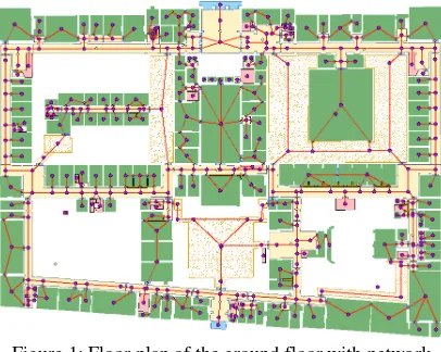
Figure 1: Floor plan of the ground floor with network visualization.
In this model, each room is first transformed into a node, forming a topologically sound connectivity model. Afterwards, this network is transformed into a geometric model by creating a subgraph for linear phenomena (e.g. corridors), as such enabling network analysis (Fig. 1). The position of the node within the room is chosen to be the geometrical center point of the polygons defining the rooms. This premise implies that the actual walking pattern will sometimes not be conform to the connectivity relationships in the network inducing small errors in the calculations of shortest and least risk paths. We will need to verify whether this error is significant in the total cost of certain paths. The selection of corridors to be transformed into linear features is based on the map text labels indicating corridor functionality. These areas also appear to be perceived as corridors when inspecting the building structure itself in the field. Obviously, this topic is depending on personal interpretation and choice. Therefore, in a future part of this research, the dependency of the performance of cognitive algorithms on the indoor ISPRS Annals of the Photogrammetry, Remote Sensing and Spatial Information Sciences, Volume II-4/W1, 2013
network topology will be investigated. This will also include testing various other indoor models, like grids and meshes.
4. ANALYSIS OF LEAST RISK PATHS IN INDOOR SPACE
In this section, a case study within our selected indoor building is analyzed on several levels: comparisons between LRP and SP algorithms in indoor space, comparison to their outdoor variants and for some preselected path a more in-depth analysis using a benchmark parameter set.
4.1 Selecting a benchmark parameter set for analysis
The goal of the LRP algorithm is to minimize the risk of getting lost. However, it is not clearly stated what a ‘minimal’ risk exactly signifies. In the original algorithm, the main parameters used to quantify and minimize ‘total risk’ are the length of each individual segment and a risk value, both weighted 50%. This raises the question on how to determine which path is actually less risky compared to other paths and on how to quantify the improved minimization in risk in the adjusted algorithm, without using the parameters defined in the algorithm itself. Several methodologies could be suggested as solutions, ranging from actual testing the accurateness with real test persons, to simulating the wayfinding problems in an agent-based environment. In this paper, we opted to select a benchmark of objective parameters that contribute to the quantification of the risk of getting lost based on research of wayfinding literature (both in indoor and outdoor space). Only those parameters are selected which are objectively linked to the spatial building structure itself. Note that the first 2 parameters are part of the algorithm itself and as such will not be used further in the benchmark parameter set.
- Risk value, i.e. more or less coinciding with the average length of taking the wrong streets at an intersection.
- Route efficiency, sometimes referred to as total path length (Hölscher et al., 2011).
- Route complexity, i.e. number of turns and number of streets used (Hölscher et al., 2011).
- Number of curves. In wayfinding, the direction strategy continuously minimizes the angle between destination and current position (Hölscher et al., 2011). However, we assume unfamiliar users which mostly follow a planned strategy. Also, in an indoor environment it is even harder to assume indoor orientation and good visibility of the destination. On the other hand, more familiar users might deviate from path, so it would be better to have a path with fewer curves. People also might feel more at ease navigating paths with fewer curves.
- Width of the corridor. Wide streets are considered more salient (Hölscher et al., 2011). Equivalent in indoor space, the selection of wider corridors can be important to reduce the risk of getting lost.
- Redundancy, i.e. a decrease in decision points that the user has to pass. Fewer nodes to make wrongful decisions at have proven to decrease wayfinding difficulties (Peponis et al., 1990).
- Integration value quantifies to what extent each space is directly or indirectly connected to other spaces. People naturally move to the most integrated nodes when navigating through a building (Peponis et al., 1990).
- Probability of path choice at an intersection, i.e. the weighing of which paths are most likely to be taken. An
uneven distribution of probability exists at each intersection, especially given the fact that more integrative spaces naturally gather more people (Peponis et al., 1990).
- Number of visible decision points. Unfamiliar participants during the initial exploration of a building, rely mostly on local topological qualities, such as how many additional decision points could be seen from a given node (Haq & Zimring, 2003).
As the individual importance and weighing of the parameters still has to be decided on, we currently use this benchmark set as a way to analyze several example routes that have been calculated (see section 4.2.2). A more elaborate evaluation has been planned as future work and as input for adjusting the initial cognitive algorithm.
4.2 Analysis of least risk paths within indoor space
4.2.1 Analysis of the entire dataset: The entire dataset consists of more than 600 nodes and more than 1300 edges. This required a computation of almost 800.000 paths to exhaustively calculate all possible paths between all nodes for both the SP and LRP algorithm.
As stated before, we would like to investigate whether least risk paths have a similar advantage to shortest paths in terms of navigational complexity as in outdoor space. Given the definition of least risk paths, we put forward the following hypotheses:
1. Length(LRP) Length(SP): measure of detour for the wayfinder for choosing a path that is less difficult to get lost on.
2. RV(LRP) RV(SP): least risk paths will more likely take routes with fewer intersections and longer edges. The shortest path will go for the most direct option ignoring the complexity of the individual intersections. 3. TotalRV(LRP) TotalRV(SP): minimization criterion
for the LRP algorithm.
Above aspects are analyzed in the following paragraphs by comparing paths calculated by both the LRP and SP algorithm. These results aim to provide an indication of the balance struck by the different algorithms between the desire for direct routes and less risky routes.
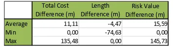
On average, the difference in path length for least risk paths is around 4,5m with a decrease in risk value of 15,5m. These values (Fig. 2) align with the hypothesis stated before, with an increase in risk values for shortest paths and an increase in path length values for least risk paths.
Total Cost Difference (m)
Length Difference (m)
Risk Value Difference (m)
Average 11,11 -4,47 15,59
Min 0,00 -74,63 0,00
Max 135,48 0,00 145,73
Figure 2: Comparison of the results of LRP versus SP algorithm over the entire indoor dataset.
Over the entire dataset, a least risk path is on average 4% longer than its respective shortest path. Although 55% of least risk paths are longer than the shortest paths, the majority (almost 99%) of the paths are less than a quarter longer. A classification of the path differences between shortest and least risk paths is shown in Fig. 3.
LengthIncrease Nr of paths % of total paths
Equal 161613 46,74%
5% or > 96491 27,90%
10% or > 45718 13,22%
25% or > 4522 1,31%
50% or > 159 0,05%
Total 345785 100,00%
Figure 3: Classification of paths
The average path lengths of the shortest and least risk paths were almost equal (109,22m to 113,69m with standard deviations of 45,89m and 48,74m respectively), intensifying the found limited differences on a whole between shortest and least risk paths in indoor spaces.
Fig. 4 summarizes the entire data set of paths and its individual differences. More specifically, it visualizes the spatial distribution of the standard deviation for all least risk paths starting in that point. The standard deviations have been classified in five quintiles, similar to Duckham and Kulik’s (2003) analysis. The figure shows generally low standard deviations (blue data points) on the first floor and in lesser connected areas of the building. The higher standard deviations (dark red data points) generally occur on the ground floor in denser connected areas and around staircases both on the ground and first floor. This greater variability can be interpreted as a result of the deviations of the least risk path from the shortest path being more pronounced at the rooms with many options like around staircases where paths can be significantly different in the final route. Starting locations within isolated areas (e.g. on the first floor) have no option but to traverse similar areas to reach a staircase and deviate from there onwards. Note that at this point elevators are not included in our dataset.
Figure 4: Spatial distribution of the standard deviation of normalized least risk path lengths (floor 0 (top) and 1
(below))
The ground floor standard deviations are generally larger due to a network with higher complexity and connectivity. This
trend can also be detected in the classification of the paths and their respective increase in length by choosing a less risky road. 80% of least risk paths with a length increase of 50% or more are found on the ground floor, while half of the paths on the first floor are equal to their respective shortest path.
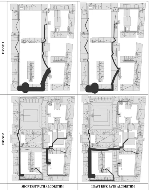
4.2.2 Analysis of selected paths: In this section, a few example paths are highlighted for further analysis. In Fig.5, an example shortest and least risk path is calculated and visualized, showing a significant difference in path choice. Both the starting and the end point are on the ground floor of the building.
Figure 5: Comparison of a typical shortest and least risk path
We used the previously defined benchmark parameter set to further analyze the differences between the LRP and SP in this example (Fig. 6). For the parameters used in the algorithm itself, the results are as expected: the total risk value for the least risk path is lower compared to the SP algorithm with a considerable lower risk value at the decision points. The least risk path is 43% longer than the shortest path, which minimizes its total length. For all the other benchmark parameters, the LRP algorithm performs worse in terms of choosing less risky edges. For example, the shortest path has 7 turns in its description, while the least risk path requires 12 turns. The number of curves in the total route is also higher in the result of the LRP algorithm. The chosen corridors in the LRP algorithm are generally less integrated, with less visibility towards the next decision points and a higher route complexity.
Figure 6: Comparison of the parameters between an example shortest and least risk path
These results indicate a less comfortable (and much longer!) route traversing for unfamiliar users compared to the shortest path which completely undermines the initial intentions of the LRP algorithm to produce easier and less risky roads. This is a perfect example of why the LRP algorithm might need to be differently implemented especially in indoor spaces.
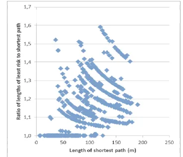
A comparison of the lengths of the least risk and shortest paths for one set of paths from a single source to every other vertex in the data set is shown in Fig. 7. The figure provides a
Shortest path algorithm
Least risk path algorithm Risk values of decision points (average; m) 274,27 166,36 Risk value of the entire path (m) 445,07 411,79 Route efficiency (length of path segments; m) 170,80 245,43 Route complexity (number of turns) 7 12 Route complexity (number of streets) 6 13
Number of curves 0 3
Width of corridors (m) 3,2 3,2 and 2
Redundancy 29 37
Number of visible decision points at each decision point (average) 5,17 4,68
scatter plot of the normalized least risk path length (the ratio of least risk to shortest path lengths), plotted against shortest path length. In this example, more than 98% of the least risk paths are less than 50% longer than their corresponding shortest paths.
Figure 7: Graph of the ratio of least risk on shortest path length to the shortest path length
Most paths are (almost) similar in length to its shortest path equivalent. Often only a small change in path choice can be found with a difference of only a couple of nodes compared to the shortest path. On the other hand, the strongly correlated stripes going from top left to bottom right in the graph exhibit blocks of correlated paths with very similar path sequences throughout their entire route. These occur because many adjacent nodes are required to take similar edges to reach their destination. This can also be seen in Fig. 5. The nodes within the dashed rectangle all take the same route for both their least risk and shortest path, resulting in connected ratios in Fig. 7.
4.2.3 Analysis of path sequences: In previous analyses, the overall differences in path length and risk value have been compared. In this section, we focus on the actual paths themselves in more detail, by trying to calculate the correlation of the entire route between shortest and least risk paths. How much alike or different are the actual paths in terms of node and edge use?
In a first analysis, we calculated for each edge the number of times all paths from a certain source node pass by this edge and this for both the SP and the LRP algorithm. The result is a map showing the use of each edge by varying line thickness. As an example, Fig. 8 (at the back of the paper) shows this calculation for all paths starting in source node 1086 (a room in the upper left corner on the first floor). This map shows a significant difference in the resulting choice of paths between SP and LRP algorithm, even though the average path length and risk value difference is respectively limited to 7,7m and 13,9m which is in line with the limited differences found over the entire dataset. More in detail, in the Dijkstra case, from the source node a large amount of paths stay on the first floor to go to a more southern located staircase and deviate from there to the specific rooms. For the LRP algorithm, to access the same nodes in the southern part of the building on the ground floor, a large amount of paths immediately descend to the ground floors and choose a specific corridor and outdoor area to find their way through the building. Additionally, nodes that have limited path choice generally take the same path in both cases (for example the northeast corner and middle/middle-east corridor
on 1st floor). This effect was also visible in the scatter plot (Fig. 7). Remarkable are the similar choices in paths for areas in the southwestern corner of the ground floor that take the same staircase. These results imply that the location of the stairs is of major importance in the selection of the paths.
In a second analysis, we computed the number of nodes that are equal between shortest and least risk path for each node to a certain source node (i.e. the Jaccard similarity coefficient for each path). The result is the ratio of the number of equal nodes divided by the total number of nodes of the respective path for the Dijkstra algorithm. Fig. 9 shows the Jaccard index for paths with source node 1086.
Figure 9: Jaccard index showing the path differences in usage of nodes (floor 0 (top) and 1 (below))
The results confirm the previously mentioned importance of stairs in path choice. Also, areas that are alike in path flow have similar ratios. A low equality of nodes can be found on the ground floor (southern middle part) as the paths take a significant different route (use of different staircase). A surprising low equality can also be found on the first floor (south middle part) which is not entirely visible on the flow map due to the small amount of paths in that area. The results from both analyses also confirm the fact that neighboring nodes often have similar path structures (with here and there a single boundary node difference). Also, the distance to the source node influences to a certain degree the path differences found in this comparison.
4.3 Analysis of indoor least risk paths compared to the results in outdoor space
In this section, we want to investigate whether our results of the calculations in indoor space are similar to those from outdoor space.
A comparison with the result obtained by Grum (2005) is difficult as the author only calculated a single path in outdoor space. In both the indoor and outdoor examples, the total risk value for the least risk path is minimal and the length is longer than its shortest path. The outdoor least risk path is 9% ISPRS Annals of the Photogrammetry, Remote Sensing and Spatial Information Sciences, Volume II-4/W1, 2013
longer than the shortest path, while in our dataset an average increase of 4% is detected. Applying the benchmark set to several indoor examples revealed riskier paths when using the LRP algorithm (compared to SP algorithm indoor), while the least risk path in the outdoor dataset is indeed the less risky choice applying the benchmark analysis. An explanation could be that the author only works with a limited outdoor dataset. Also, the least risk path indoor might have a different connotation because of the description of the indoor network. Due to the transformation of the corridor nodes to a linear feature with projections for each door opening, the network complexity is equivalent to a dense urban network. However, the perception for an indoor wayfinder is totally different. While in outdoor space each intersection represents a decision point; in buildings, the presence of door openings to rooms on the side of a corridor is not necessarily perceived as a single intersection where a choice has to be made. Often these long corridors are traversed as if they were a single long edge in the network.
Simplest paths have similarly to least risk paths the idea of simplifying the navigation task for people in unfamiliar environments. The cost function in both simplest and least risk paths accounts for structural differences of intersections, but not for functional aspects (direction ambiguity, landmarks in instructions…) like the simplest instructions algorithm (Richter & Duckham, 2008). However, the simplest path algorithm does not guarantee when taking one wrong decision that you will still easily reach your destination, while the LRP algorithm tries to incorporate this with at the same time keeping the complexity of the instructions to a minimum. Several of the comparison calculations are similar to the ones calculated for simplest paths (Duckham & Kulik, 2003). At this point, we cannot compare actual values as it covers a different algorithmic calculation. In the future, we plan to implement the simplest path algorithm also in indoor spaces. However, it might be useful at this point to compare general trends obtained in both.
With regard to the variability of the standard deviations (Fig. 4) similar conclusions can be drawn. At the transition between denser network areas and more sparse regions, the variability tends to increase as a more diverse set of paths can be calculated. The sparse and very dense areas have similar ratios showing similar network options and path calculations. The case example can also be compared to a worst-case dataset of the outdoor simplest path. A similar trend in ‘stripes’ as found in the graph in Fig. 7 is also found in the outdoor simplest path results, also due to sequences of paths that are equal for many adjacent nodes (Duckham & Kulik, 2003).
5. RECOMMENDATIONS FOR ADJUSTING THE LEAST RISK PATH ALGORITHM
The previous analyses have shown multiple times that the calculated least risk paths are actually not less risky than its shortest path equivalent in indoor environments. Therefore, adjustments to the original definition of the algorithm are required to be more in line with the indoor situation. These will be tested in future research as to result in a more cognitively accurate algorithm for wayfinding in indoor spaces.
Currently, the risk value of a decision point is calculated based on the assumption that the wayfinder recognizes his
mistake at the first adjacent node and returns from there to the previous node. However, is it actually realistic that people already notice at the first intersection that they have been going wrong? An increasing compounding function could be suggested taking into account the possibility of going further in the wrong direction. Also, depending on the environmental characteristics, the chances of noticing a wrong decision can change dramatically. For example, signage and landmarks can help, but there appearance and understanding by the user is highly unpredictable. Additionally, the fact that you have to walk up and down staircases (or taking an elevator) could be naturally having a greater weight because taking a wrong decision might result in walking up and down the stairs twice. On the other hand, chances of taking a wrong decision by changing floors are likely to be slimmer given the effort for vertical movement and a changed cognitive thinking.
In line with this last point, wayfinding research (Hölscher et al., 2009) has shown that people’s strategy choice indoors varies with different navigation tasks. Tasks with either a floor change or a building part change result in no problems, with the participants first changing to the correct floor or building part. However, for tasks with changes in both vertical and horizontal direction, additional information is required to disambiguate the path choice. An algorithm that wants to minimize the risk of getting lost necessarily needs to account for these general indoor wayfinding strategies as they correspond to the natural way of multilevel building navigation for all types of participants.
In the current implementation of the LRP algorithm, both the length of the path as well as the sum of the risk values at intermediate decision points have an equal weight in the calculation of the total risk value. Varying the individual weight of both parameters might results in a more cognitively correct calculation of the indoor least risk paths. Also, a more sophisticated algorithm could select routes that preferentially use more important or higher classified edges.
As previously mentioned, the description of the indoor network has a large influence on the results of the least risk comparisons. The introductions of many dummy nodes in front of doors that are not perceived as intersections, introduces a complexity in the risk value calculation, which seems to heavily influence our results. Therefore, the second stage of this research will investigate the importance and size of this dependency of the performance of cognitive algorithms on the indoor network topology.
6. CONCLUSIONS
In this paper, the LRP algorithm as developed by Grum (2005) in outdoor space is implemented and tested in an indoor environment. Analyses on our indoor dataset revealed the following conclusions. First, only a limited average increase in path length is found compared to the shortest paths in return for theoretically less risky paths. Second, deviations from the least risk path compared to the shortest path were mostly recognized at nodes with many decision points (e.g. around staircases). Those staircases appeared to be also of major importance for the selection of paths in the correlation analysis. Third, a benchmark parameter set was deducted from wayfinding literature to objectively qualify the ‘riskiness’ of the least risk paths. Several examples have proven that the least risk path is not necessarily less risky than its shortest path equivalent. On the contrary, in one of ISPRS Annals of the Photogrammetry, Remote Sensing and Spatial Information Sciences, Volume II-4/W1, 2013
the examples, the shortest path would still be preferred over the least risk path. Fourth, comparisons of our results to the outdoor variant are difficult due to limited data outdoor. However, a similar increase in length has been found.
Our main conclusions from the analyses indicate that improvements to the indoor variant of the LRP algorithm are necessary, given the complexity of the current least risk paths. Changes in the calculation of the risk value, together with a weighing of the parameters will be tested. The benchmark parameter set will be implemented to test more paths in the future and will also be used to adjust and compare the improvements to the improved LRP algorithm. Finally, the influence of the network structure will be investigated in future research in a search for optimizing the algorithm to be more compliant to the cognitive notion of indoor wayfinding.
7. REFERENCES
Atila, U., Karas, I., & Rahman, A. (2013). A 3D-GIS Implementation for Realizing 3D Network Analysis and Routing Simulation for Evacuation Purpose. In J. Pouliot, S. Daniel, F. Hubert & A. Zamyadi (Eds.), Progress and New Trends in 3D Geoinformation Sciences (pp. 249-260): Springer Berlin Heidelberg.
Cherkassky, B., Goldberg, A., & Radzik, T. (1996). Shortest paths algorithms: Theory and experimental evaluation. Mathematical Programming, 73(2), 129-174.
Dijkstra, E. W. (1959). A Note on Two Problems in Connexion with Graphs. Numerische Mathematik, 1(1), 269-271.
Duckham, M., & Kulik, L. (2003). “Simplest” Paths: Automated Route Selection for Navigation. In W. Kuhn, M. Worboys & S. Timpf (Eds.), Spatial Information Theory. Foundations of Geographic Information Science (Vol. 2825, pp. 169-185): Springer Berlin/Heidelberg. Fu, L., Sun, D., & Rilett, L. R. (2006). Heuristic shortest path
algorithms for transportation applications: State of the art. Computers & Operations Research, 33(11), 3324-3343. Grum, E. (2005). Danger of getting lost: Optimize a path to
minimize risk. Paper presented at the 10th International Conference on Information & Communciation Technologies (ICT) in Urban Planning and patial Development and Impacts of ICT on Physcial Space, Vienna, Austria.
Haq, S., & Zimring, C. (2003). Just Down The Road A Piece: The Development of Topological Knowledge of Building Layouts. Environment and Behavior, 35(1), 132-160. Hölscher, C., Büchner, S. J., Meilinger, T., & Strube, G.
(2009). Adaptivity of wayfinding strategies in a multi-building ensemble: The effects of spatial structure, task requirements, and metric information. Journal of Environmental Psychology, 29(2), 208-219.
Hölscher, C., Tenbrink, T., & Wiener, J. M. (2011). Would you follow your own route description? Cognitive strategies in urban route planning. [Article]. Cognition, 121(2), 228-247.
Lee, J. (2004). A Spatial Access-Oriented Implementation of a 3-D GIS Topological Data Model for Urban Entities. Geoinformatica, 8(3), 237-264.
Li, K.-J. (2008). Indoor Space: A New Notion of Space. In M. Bertolotto, C. Ray & X. Li (Eds.), Web and Wireless Geographical Information Systems (Vol. 5373, pp. 1-3): Springer Berlin/Heidelberg.
Mautz, R., Kunz, M., & Ingensand, H. (2010). Abstract Volume of the 2010 International Conference on Indoor Positioning and Indoor Navigation. Zurich, Switzerland. Musliman, I. A., Abdul-Rahman, A., & Coors, V. (2008).
Implementing 3D network analysis in 3D-GIS. Paper presented at the 21st ISPRS Congress Silk Road for Information from Imagery, Beijing, China.
OGC. (2013). OGC IndoorGML (Vol. OGC 13-nnnrx - Version: v.0.8.0, pp. 72).
Peponis, J., Zimring, C., & Choi, Y. K. (1990). Finding the Building in Wayfinding. Environment and Behavior, 22(5), 555-590.
Richter, K.-F., & Duckham, M. (2008). Simplest Instructions: Finding Easy-to-Describe Routes for Navigation. In T. Cova, H. Miller, K. Beard, A. Frank & M. Goodchild (Eds.), Geographic Information Science (Vol. 5266, pp. 274-289): Springer Berlin/Heidelberg.
Vanclooster, A., Neutens, T., Fack, V., Van de Weghe, N., & De Maeyer, P. (2012). Measuring the exitability of buildings: A new perspective on indoor accessibility. Applied Geography, 34(0), 507-518.
Vanclooster, A., De Maeyer, P., Fack, V., & Van de Weghe, N. (2013). Calculating least risk paths in 3D indoor space. Paper presented at the 8th 3D GeoInfo conference, Istanbul, Turkey.
Viaene, P., & De Maeyer, P. (2013). Detecting landmarks for use in indoor wayfinding. Ghent University, Ghent. Walton, L. A., & Worboys, M. (2009). Indoor Spatial
Theory.
www.spatial.maine.edu/ISAmodel/documents/IST_ISA0 9.pdf
Worboys, M. (2011). Modeling Indoor Space. Paper presented at the Third ACM SIGSPATIAL International Workshop on Indoor Spatial Awareness (ISA 2011), Chicago, IL.
8. ACKNOWLEDGEMENTS AND APPENDIX
Financial support from the Flanders Research Foundation (FWO-Vlaanderen) is gratefully acknowledged.
This paper is based on an initial conference paper, accepted for the 8th 3D GeoInfo conference in Istanbul. However, it has been updated with the latest research results.
F
LO
O
R
1
F
LO
O
R
0
SHORTEST PATH ALGORITHM LEAST RISK PATH ALGORITHM