USING SEMANTIC DISTANCE TO SUPPORT GEOMETRIC HARMONISATION OF
CADASTRAL AND TOPOGRAPHICAL DATA
M. J. Schulze*, F. Thiemann, M. Sester
Institute of Cartography and Geoinformatics, Leibniz Universität Hannover, Germany - {schulze, thiemann, sester}@ikg.uni-hannover.de
Technical Commission II
KEY WORDS: GIS, Adjustment, Matching, Harmonisation, Automation
ABSTRACT:
In the context of geo-data infrastructures users may want to combine data from different sources and expect consistent data. If both datasets are maintained separately, different capturing methods and intervals leads to inconsistencies in geometry and semantic, even if the same reality has been modelled. Our project aims to automatically harmonize such datasets and to allow an efficient actualisation of the semantics. The application domain in our project is cadastral and topographic datasets. To resolve geometric conflicts between topographic and cadastral data a local nearest neighbour method was used to identify perpendicular distances between a node in the topographic and an edge in the cadastral dataset. The perpendicular distances are reduced iteratively in a constraint least squares adjustment (LSA) process moving the coordinates from node and edge towards each other. The adjustment result has to be checked for conflicts caused by the movement of the coordinates in the LSA.
The correct choice of matching partners has a major influence on the result of the LSA. If wrong matching partners are linked a wrong adaptation is derived. Therefore we present an improved matching method, where we take distance, orientation and semantic similarity of the neighbouring objects into account. Using Machine Learning techniques we obtain corresponding land-use classes. From these a measurement for the semantic distance is derived. It is combined with the orientation difference to generate a matching probability for the two matching candidates. Examples show the benefit of the proposed similarity measure.
* Corresponding author.
1. INTRODUCTION
Reliable vector databases play an important role in various applications and activities. National mapping agencies provide data, as topographic datasets of different resolutions, often also cadastral datasets. In Germany, the topographic and the cadastral data are acquired independently using different techniques and they are also maintained independently. As these processes are somehow redundant, the two databases should be harmonized to reduce the costs for maintaining and updating both databases.
The German cadastral database, called ALKIS, is based on a reference scale of 1:1.000 and represents all land parcels in the form of polygons to build a reference to their ownership. To acquire data for this database mainly terrestrial local measurements, like tachymetry, are used to obtain vector data with high accuracy and density. These measurements are triggered on certain change events such as splitting up a land parcel.
The German topographical database, referred to as ATKIS, is based on a reference scale of 1:10.000. Due to the smaller scale, several certain objects are represented as polyline features, like road- or river networks. Several acquisition techniques are used for updating this database which can be classified as more global overview, like aerial images or changes in the restrict use of parcels. As polygons in this database do not represent the corresponding land parcels, but their usage, several parcels in ALKIS could be aggregated to form one polygon in ATKIS. The updating of this topographical database is triggered in given time cycles to obtain a harmonic actuality.
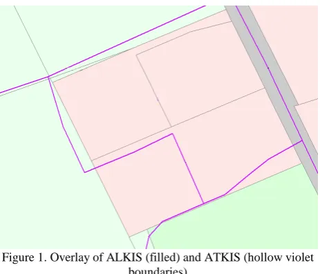
Overlaying the two representations of topographic and cadastral objects reveals differences in the objects (see Figure 1).
Figure 1.Overlay of ALKIS (filled) and ATKIS (hollow violet boundaries)
These differences can be explained by the following factors: - Different scale, resulting in different geometric
resolution; this leads to a different density of points describing an object, and also different accuracies - Different scale, resulting in different semantic
resolution, also leading to different classification schemes: in ATKIS there are object classes describing mixed usage (e.g. settlements, vegetation)
- Different data models: e.g. in ATKIS roads are modelled as lines, whereas in ALKIS they are represented as polygons
- Different definition of objects: whereas in ALKIS the property plays a major role, thus, the usage of individual properties is described; in ATKIS the topographic aspect is highlighted. This leads e.g. to the effect that in ATKIS a lake is defined by the water body, whereas in ALKIS also the surrounding shore is included.
- Errors in data capture
- Differences due to different acquisition time
The specifics in the problem addressed in the paper is that the goal is to have a consistent and visually convincing result, where parts of object boundaries of corresponding objects which are in a local vicinity do match. Thus, it is not required that a whole object is adapted, but only parts of the object boundaries, which are close to each other. This leads to the following problem:
- Given two datasets with partially corresponding object boundaries
- Fuse common boundaries, which likely correspond to the same object and which are close to each other
This leads to a matching approach, which analyzes correspondences between objects locally, on a point-to-line basis. An integrated linear equation system is set up which establishes correspondences between all points of an object to possible corresponding lines of the other datasets. The equation system is solved by Least Squares Adjustment. The decision concerning a possible correspondence is taken based on the following similarity criteria:
- Distance between objects
- Local geometric similarity (direction of lines) - Similarity of neighbouring object classes
In this paper, the focus lies on the determination of valid local correspondences between object parts. To this end, a learning method is proposed, which analyzes existing datasets and extracts probable correspondences. In addition, also relations of object in the local environment of the objects are used, e.g. following section, the approach is applied to different datasets to show its potential. The paper concludes with a summary and an outlook on future work. corresponding features in both datasets: simpler approaches just look at objects in the spatial vicinity, whereas more complex methods also take the relations of the objects into account (Walter & Fritsch 1999). Li and Goodchild (2010) proposed a holistic approach for matching based on linear programming. Harvey & Vauglin, 1996, address the problem of alignment and propose a statistical approach to determine thresholds for geometric variations of geometries, which leads to multiple
thresholds. These measures take geometric and semantic accuracy into account. Using semantics as similarity criterion presumes that semantic correspondences between the objects in the different datasets are known – otherwise, they have to be determined (see e.g. Duckham & Worboys, 2005; Kieler et al. 2007). Some approaches target at matching data from different scales (Mustière & Devogele, 2008; Kieler et al., 2009). Most approaches target at transforming objects from one dataset to the other using a rigid transformation (Sester et al., 1998). In addition, there are methods which use rubber sheeting approaches in order to homogenize corresponding objects (Doytsher et al., 2001, Siriba et al. 2012). Kampshoff and Benning (2005) use Least Squares Adjustment to harmonize data, which allows including specific constraints, such preservation or enhancement of right angles or areas. Butenuth et al., 2007, propose a flexible adaptation of corresponding features, and to determine quality and reliability parameters of the result.
3. APPROACH
The algorithm to match corresponding objects and eliminate the geometric inconsistencies consists of four steps: First the correspondences between the two datasets from nodes in one dataset to close by line segments in the other are established. Then a similarity indicator for each link is calculated, based on which in the next step the most promising links are selected. In the last step the selected links are used to minimize the geometric inconsistencies in a least squares adjustment process. In this section, we describe all of these four steps.
3.1 Finding correspondences
Due to scale and modelling differences, objects in the two datasets are represented in different dimensions. This holds true for slim and elongated objects such as roads and rivers: in the topographic dataset, they are modelled as lines (if their width is below a certain value), whereas they are modelled as polygons in cadastre. The other objects (e.g. settlement or vegetation areas) are modelled as polygons in both datasets.
To eliminate the geometric inconsistencies the strategy described in (Dalyot et al. 2012) is based on finding geometric correspondences between two datasets and eliminating the geometric difference via a constraint least squares adjustment method (LSA). The correspondences are build via the perpendicular distance from a line segment PiPi+1 in one dataset x1, with a given covariance matrix xx,1, to a point Pj in the other dataset x2, with the given covariance matrix xx,2. This constellation is shown in Figure 2. To define whether a found correspondence is valid or not, two geometric thresholds are used: the perpendicular distance dij, which must not exceed a given length and the projection of the point to the line segment pij, for which small extrapolations beyond the boundaries of a line segment are allowed. In addition, the orientation angle ij of the line segment is determined (Equation 1 and 2), which is also used later in the LSA process.
A slightly different strategy is needed for creating links between polygons and corresponding polylines, where the polylines are regarded as the middle axis of the polygons. This situation
occurs, when data from different scales have to be integrated, where linear objects are modelled as polygons in the large scale dataset and as polylines in the other. In this case two links in
Figure 2. Correspondences between two polygon features
correspondences build on the two thresholds for pij and dij alone are not reliable enough to be used in the LSA. Non correct links in the LSA not only lead to wrong adaptations between the two datasets, they also lead to topological errors like self intersecting objects and shifts with very high displacement values, that are exceeding the proportion of the geometric conflict.Therefore we must take additional criteria into account to find reliable correspondences between the datasets.
In this paper we therefore present the approach of using semantics in addition to the geometric threshold values to create more reliable correspondences. In German cadastral and topological datasets every object carries attributes with its semantic description. These descriptions are the same in both datasets, but can be different for the same real world object due to different capturing techniques, different generalisation, interpretation and actuality. Therefore we use a Machine Learning approach, described in the next section, to determine a probability for corresponding pairs of objects in the two datasets.
3.2 Similarity indicator based on semantic information
A segment segregates a pair of land-use classes – which may also be identical. Semantically identical segments segregate two corresponding pairs of land-use classes.
However, due to the semantic differences of both datasets, it is not given, that the land-use classes of corresponding objects are identical (see Figure 3). Therefore, the goal is to link similar land-use objects.
As described before, a link connects a line segment from the first dataset with a node from the second dataset. The node is adjacent to a set of two or more segments (see Figure 4). The aim is to identify if there is a segment in the second dataset that
is similar in direction and semantics to the segment in the first dataset. If this is the case, the chance of having found two corresponding elements is high.
Figure 3: Comparison of the land-use in the cadastral and topographic dataset: Objects of different land-use domains are
displayed in dark red, with same domain in light red and with identical classes in white.
Figure 4. Linked node and adjacent segments. The similarity indicator determines the best matching segment (bold), which links the B-A segment in the blue dataset with a B-A segment in
the red one.
The calculation of the similarity indicator consists of two steps: first, the calculation of the semantic similarity of land-use classes as pre-process and second, the derivation of segment and link similarities based on the semantic similarity.
3.2.1 Semantic similarity of land-use classes
The first step of our approach is to learn the corresponding land-use classes. For that purpose we intersect the two datasets. To consider only corresponding polygons and reduce the influence of geometric discrepancies we filter the intersection result. Intersection polygons smaller than nine square meters or with an overlap smaller than 1 % of the larger and 67 % of the smaller input polygon are removed. Also – as described above – cadastral objects with classes that correspond to linear geometry in the topographic dataset are not regarded in the process.
ATKIS
Table 1. Small part of the confusion matrix. The fields contain the summed up areas in hectare. Each line corresponds to a
cadastral class, each row to a topographical class.
For the remaining polygons we sum up the areas in a pivot table to get a confusion matrix with rows for each cadastral and columns for each topographic land-use class (an extract of the matrix is given in Table 1). For an unambiguous assignment the confusion matrix would be a diagonal one. In our case we have some well matching classes (e.g. lakes and rivers) and not matching classes (e.g. grove). Other classes are segregated with a given uncertainty. In this example the residential and
commercial areas have the maximum values in the diagonal element, but also a significant part matches to mixed used areas in the topographic dataset. The really rare mixed used areas in cadastral data mostly match to mixed used areas in topographic data. But in the topographic dataset a much larger fraction exits that is generated by aggregation of smaller residential and commercial areas. The diagonal element of mixed use is small referring to the fraction of mixed use in the topographic dataset and large referring to the fraction in the cadastral dataset.
min CT CT
C T
A P
A A
(3)
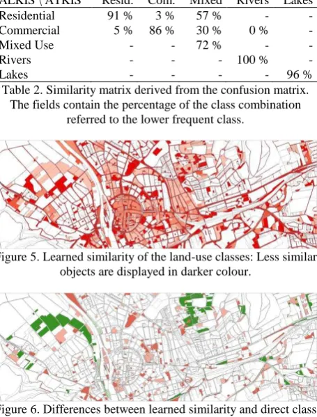
As similarity measure the percentage of the combination (PCT) calculated from the area of the combination (ACT) divided by the smaller value from the area of the cadastral class (AC) and the topographic class (AT) is used. The minimum function is used, because the combination of the two classes cannot occur more often than the smaller partition of the combined classes. The similarity values for the example from Table 1 are shown in Table 2. Figure 5 visualizes the similarities from the complete sample dataset. A significant part of the features regarded as incompatible by the direct comparison were identified to be matching classes after the learning process (dark green features in Figure 6).
ALKIS \ ATKIS Resid. Com. Mixed Rivers Lakes
Residential 91 % 3 % 57 % - -
Commercial 5 % 86 % 30 % 0 % -
Mixed Use - - 72 % - -
Rivers - - - 100 % -
Lakes - - - - 96 %
Table 2. Similarity matrix derived from the confusion matrix. The fields contain the percentage of the class combination
referred to the lower frequent class.
Figure 5. Learned similarity of the land-use classes: Less similar objects are displayed in darker colour.
Figure 6. Differences between learned similarity and direct class comparison (green/red – feature similarity higher/lower)
3.2.2 Segment similarity
In this step a segment similarity indicator will be derived from the semantic similarity of the left and right pairs of land-use classes. First it is to decide which sides of the segments are corresponding. This is obvious when the two segments are parallel. In case of the direction being opposite, the left side is corresponding with the right side and vice versa. For orthogonal segments it is not possible to decide which sides are
corresponding and for nearly orthogonal segments the assignment is very uncertain. The semantic similarity of two segments is calculated as average of the similarities (PCT) of the left and the right land-use pairs. To take the directional similarity into account, we scale the semantic similarity with the absolute value of the cosine of the angular difference of both segments (∆α).
1
cos 2
l r
seg CT CT
P P P (4)
As result we have the following behaviour: Orthogonal segments are not similar, parallel segments with matching land-uses in both datasets on left and right side are most similar. If left and right land-use pares do not match the similarity is also null. If only one pair matches a fair similarity value is calculated.
Finally, the semantic similarity of the link is determined as the semantic similarity of the best matching segments.
3.3 Filtering links based on the similarity indicator
As described in Section 3.1, the focus in this paper lies on finding and verifying the correspondences between polygon objects. The used method obtains all links from all line segments in x1 to the corresponding points in x2 that do not exceed the given geometric thresholds. For this reason several links can end in the same common node of x2. A decision method based on the length of the link is proven to be not reliable enough, as small or slim objects can have a translation error high enough to catch the opposite side of its corresponding polygon (left), or the wrong feature in general (right), as depicted in Figure 7.
Figure 7. Assignment to the opposite side of the corresponding object (left), assignment to the wrong object (right) (green
arrows: shortest links)
Therefore an additional decision strategy is used to enhance the confidence that the picked links for the adjustment are correct based on the available semantics of the datasets. For each point Pij in Dataset x2 all the links starting at this point are captured. From the semantic analysis described in section 3.2.2 a similarity indicator based on the accordance of the land-use information on both sides of the line segment in the two datasets and the correct angle is obtained. Based on this indicator it is now possible to create a ranking for all links starting in this point. Only the best link based on the indicator is chosen to be used in the adjustment process, while the rest are excluded. However there may be cases where there is only one
link starting from a point that still points on a wrong target feature and thus has a low similarity values. To take this case into account, a threshold for the similarity indicator that has to be exceeded is also used and the link is excluded from the adjustment process if there is low confidence in it.
3.4 Least squares Adjustment process
After the links have been filtered based on their similarity indicator, the least squares adjustment process is now adapted to the datasets.
Using Equation 1 we create a functional model for a least squares adjustment process based on conditional observations. The goal is to minimize the quadratic sum of the perpendicular distances dij, as we are not regarding polyline to polygon assignments, by shifting the line segment PiPi+1 of x1 and the node Pj of x2 toward each other.
To solve the mathematical problem, the functional model (1) has to be linearized to preserve the functional matrix Bx, that describes the linear dependency between the given perpendicular distances dij, regarded as contradictions wx, and the coordinates between both datasets, and the sought shifts of the coordinates vx. Bx and vx are split up intoblocks for each dataset x1 or x2 (5).
In addition, a stochastic model Qll,x can be initialized, giving the coordinates of every point that is handled in the adjustment techniques described in the introduction, there is no correlation expected between them. Also as there is no information about the correlation between points in one dataset available, so Qxx,1 and Qxx,2 are regarded as diagonal matrices.
The solution is calculated so that the quadratic sum of wx is minimized. After the solution is derived, the calculated coordinate shifts are assigned to the two datasets.
As a linearized model is used to solve the problem, several iteration steps need to be calculated until convergence is reached. Each iteration step consists of all steps mentioned before:
1. Find the links between two datasets.
2. Calculate the similarity indicator for every link and choose the best one available per point.
3. Run the least squares adjustment process. 4. Assign the coordinate shifts to the datasets.
4. EXPERIMENTAL RESULTS AND DISCUSSION
The previously described algorithm is tested using the topographic dataset (ATKIS) and the cadastral dataset (ALKIS) from the area of Hameln in Germany, Lower Saxony. The overall area of the test field from which we show several examples here is 12 km² and consists of about 4000 polygons in
the cadastral dataset and about 800 polygons in the formed by the borderline between river and grove. The issue in this case is that in ALKIS the grove is partitioned into very narrow polygons parallel to the riverbank, e.g. 976 (black) having a width of approximately 5 to 6 meters. Every polygon in ATKIS that is close to this constellation will lead to links to both sides of the polygon, but only the border between grove which point to a boundary between a pair of grove objects get a low similarity.
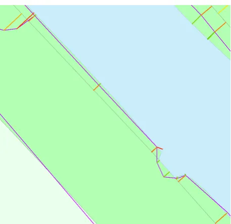
Figure 8. ALKIS (black) and ATKIS (purple) data overlay on the riverbank of Weser in Hameln. Links with similarity
indication (coloured lines)
Before the adjustment process, the best links are chosen based on the method described in section 3.3. After the adjustment, the whole process described in section 3.4 is iterating for five times in this case. It has to be mentioned that due to the higher expected geometric accuracy of ALKIS data, for each iteration step the original dataset is put in it so that the ATKIS dataset is iterating toward the boundaries of ALKIS, also the variance of the points in ALKIS is set to be an order of magnitude better in relation to ATKIS. The final result is shown in Figure 9. The ATKIS dataset is now aligned to the proper corresponding boundaries in ALKIS. However there are some areas left, where both datasets do not match perfectly. This is caused by the coarse density of the points in ATKIS, which do not allow a perfect alignment to the finer structures in ALKIS. A solution
strategy to this problem is described in (Dalyot et al. 2013) and will be adapted to this process in the future.
Figure 9. Adjustment result of Weser riverbank (test case 1)
However, all the nodes of ATKIS align to the correct corresponding line features in ALKIS. Table 3 gives a brief overview of the adjustment results. As the mean link length and the mean shift are both the same order in the last iteration and below 10 cm, we can assume to have a convergent solution.
Mean Link Length Mean Shift
First Iteration 2.74 m 1.37 m
Last Iteration 0.07 m 0.06 m
Table 3. Results for first and last iteration step for the adjustment (test case 1)
Our second test example shows the importance of evaluating not only the semantic correspondence but also the matching direction of both corresponding features. The example is given in Figure 10.
Figure 10. ALKIS (black) and ATKIS (purple) data overlay for a forest. Links with similarity indication (coloured lines)
In the lower left part of the object, there are several red links which are indicating that the confidence in them is not very high. The reason is that the boundary line in ATKIS (purple) is
fetching not only the right side of the corresponding polygon, but also the opposite side. This is detected by the similarity evaluation process and results in a low indicator. The links to the correct corresponding line segment shown in green are trusted and therefore used in the adjustment process.
To reach a stable solution for this case, 14 iterations were needed. The statistical results are shown in Table 4 and the shifted ATKIS dataset is shown in Figure 11.
Mean Link Length Mean Shift
First Iteration 3.87 m 1.84 m
Last Iteration 0.02 m 0.01 m
Table 4. Results for first and last iteration step for the adjustment for (test case 2)
In this case, the ATKIS dataset aligns almost as nicely to ALKIS as in test case 1. However apart from the alignment problem caused by the coarse density of the nodes already mentioned, the bottom left part has build a peak which is not aligning to the corresponding polygon. This is caused by a missing link to the bottom part of the ALKIS object due to the link filter only taking the best quality link available for a point. As the link to the left part always occurs to have a higher quality than the link to the bottom part, because these are almost perpendicular to each other, it is therefore judged with a lower similarity indicator.
Figure 11. Adjustment result for a forest patch (test case 2)
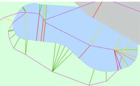
The third test case is an area around a small pond and is shown in Figure 12. Its boundaries are shifted so far apart, that the problem stated in section 3.3 appears where the links can fetch the opposite side of the matching polygon. In this case not only the semantic information but also the correct orientation of the line segment helps to identify the correct correspondence, while the wrong assignments are filtered out. This nicely underpins the relevance of the additional similarity criteria introduced in this paper – as opposed to using only a distance based criterion. To reach a stable solution of the adjustment, 22 iterations were calculated. The statistical results are given in Table 5 and Figure 13 shows the graphical presentation of the aligned dataset.
Figure 12. ALKIS (black) and ATKIS (purple) data overlay for pond area. Links with similarity indication (coloured lines)
In this case the algorithm chose the links based on the orientation of the polygon, as the matching land-use classes around the bank of the pond have to appear in the same orientation for both line segments. This leads to a nice alignment of both datasets.
Mean Link Length Mean Shift
First Iteration 5.15 m 2.57 m
Last Iteration 0.03 m 0.02 m
Table 5. Results for first and last iteration step for the adjustment for test case 3
Figure 13. Adjustment result for pond area (test case 3)
Figure 14. ALKIS (black) and ATKIS (purple) data overlay for grove area. Links with similarity indication (coloured lines)
The fourth test area is giving an example for a false positive line segment matching (see Figure 14). In the semantic correspondence matrix, a link between a grove (green) and an agricultural patch (light green) has a higher probability than a
link to a corresponding grove object. Therefore the links pointing to the borderline of neighbouring agriculture are more likely to be chosen, as shown by the green links on the lower side. Note however, that on the northern side there was no better correspondence, so the algorithms selected the less probable – solution, which in this case is the right one. Due to the indicated better similarity to the borderline of the agricultural patch, the algorithm tends to trust these links more than the correct ones resulting in the borderline of the patch being pulled to the bottom polygon, as depicted in Figure 15. The reason for this wrong assignment is shown in Table 6. The table showing the property of corresponding land-use classes in both datasets shows that the correspondence of grove to grove patches in both datasets is rarely appearing. So the correspondence probability of grove land to other classes like agriculture or barren patches is almost an order of magnitude higher, leading to an uncertain decision of which links to use. This erroneous adaptation is due to the untypical situation – which was not represented in the training data. The result reflects the most probable situation, which still can be the wrong solution! Still, one could argue that the visually disturbing sliver polygons have been reconciled.
ALKIS \ ATKIS Agriculture Grove Barren
Agriculture 99 % 35 % 26 %
Grove 16 % 5 % 52 %
Barren 28 % 51 % 47 %
Table 6. Properties for corresponding land-use classes (row: ATKIS, column: ALKIS)
Figure 15. Adjustment result for grove patch (test case 4)
5. DISCUSSION AND OUTLOOK
Using the new similarity indicator for the adjustment shows that the confidence in finding the correct corresponding links has improved significantly. The problems to fetch the correct borderline in narrow polygons have been reduced, as shown in test case 1. Also finding the correct borderline side of a corresponding polygon appears to be much more reliable, as shown in test cases 2 and 3. This was not possible by using a geometry based measure alone.
These promising results still have to be evaluated for larger datasets. Also, there are several further issues to include: e.g. the process for evaluating the similarity is now limited to a local point to line correspondence; in some cases it might be necessary to extend the field of view here and use information about neighbouring links on the same object to get a higher confidence that the right link is chosen for the adjustment process. Still, however, it has to be kept in mind that the problem is not a 1:1 feature matching, but a rather local
adaptation to the best fitting corresponding line – thus neighbouring nodes do usually have different matching features. Also the algorithm for detecting the links with the highest similarity can be improved as it now uses only the best link available for a point and employs a threshold to eliminate links of a bad similarity. This threshold, however, has to be adapted to every situation, so it still has to be evaluated for a larger dataset (e.g. in the above shown tests, different thresholds have been applied). Further, the experiments have shown that in various situations it is helpful to obtain more than one link from a point to several line segments to achieve a better fitting adjustment result. This result can also be improved by splitting up the line segments from the dataset with the coarser point density (by interpolating additional Steiner points).
Although the link similarity indicator gave good and reliable results for our test cases, there are possibilities that there are still faulty links chosen for the adjustment process, although they do have a good similarity indicator. This results from semantic differences in both datasets resulting from different actualities and interpretation while obtaining these datasets. These links lead to wrong shifts in the adjustment process and may cause unwanted collapsing geometric constellations after the adjustment process. Also significantly large shifts of a point in respect to the neighbouring ones may lead to topological errors like self intersecting polygons.
Adjustment theory allows the evaluation the results with respect to possible significant errors. To this end, data snooping and/ or robust adjustment can be integrated to improve the stability and reliability of the adjustment result.
Another issue to be addressed in the future is the fact that not all objects find corresponding partners in the other dataset. Those objects are eliminated from the whole adaptation procedure in the current approach. In order to also allow that these objects are adapted, one possibility is to apply rubber sheeting based on the vector field of the corresponding features. Another possibility is to further exploit the adjustment approach and include additional constraints between all the objects – similar to what is being done for the displacement operation in generalisation (Sester, 2005; van Dijk & Haunert, 2014). This also allows the preservation the shapes, areas, and topological relations of the features while they are adapted to their corresponding objects in the other dataset.
Overall, the link similarity indicator to improve the confidence in the link decision shown in this paper is giving good results in our test cases and gives the possibility to align two datasets in regions where a correct decision for the right correspondences is not possible based on mere geometric criteria.
6. REFERENCES
Butenuth, M., Gösseln, G. v., Tiedge, M., Heipke, C., Lipeck, U., Sester, M., 2007. Integration of heterogeneous geospatial data in a federated database. ISPRS Journal of Photogrammetry & Remote Sensing, 62, pp. 328-346.
Dalyot, S., Dahinden, T., Schulze, M. J., Boljen, J., Sester, M., 2012. Geometrical Adjustment towards the Alignment of Vector Databases. In: ISPRS Annals of Photogrammetry, Remote Sensing and Spatial Information Sciences, Vol. I-4, pp. 13-18.
Dalyot, S., Dahinden, T., Schulze, M. J., Boljen, J., Sester, M., 2013. Integrating network structures of different geometric representations. Survey Review, Vol. 45, No. 333, pp. 428-440.
Doytsher, Y., Filin, S., Ezra, E., 2001. Transformation of a datasets in a linear-based map conflation framework. In: Surveying and Land Information Systems. 61 (3), pp. 159-169.
Duckham, M., Worboys, M., 2005. An algebraic approach to automated geospatial information fusion. International Journal of Geographical Science, 19 (5), pp. 537–557.
Dijk van, T.C., Haunert, J.-H., 2014. Interactive Focus Maps Using Least-Squares Optimization. International Journal of Geographic Information Science.
Harvey, F., Vauglin, F., 1996. Geometric match Processing: Applying multiple tolerances. In: Proceedings, 7th International Symposium on Spatial Data Handling, 4A, pp. 13-29.
Kampshoff, S., Benning, W., 2005. Homogenisierung von Messdaten im Kontext von Geodaten-Infrastrukturen. ZfV Zeitschrift für Vermessungswesen, 130, pp. 133-147.
Kieler, B., Sester, M., Wang, H., Jiang, J., 2007. Semantic Data Integration: Data of Similar and Different Scales. Photogrammetrie Fernerkundung Geoinformation (PFG), Vol. 6, pp. 447-457.
Kieler, B., Huang, W., Haunert, J.-H., Jiang, J., 2009. Matching River Datasets of Different Scales. In: Advances in GIScience: Proceedings of 12th AGILE Conference on GIScience, Lecture Notes in Geoinformation and Cartography, Springer, Berlin, pp. 135-154.
Li, L., Goodchild, M.F., 2010. Automatically and accurately matching objects in geospatial datasets. In: Proceedings of theory, data handling and modelling in geospatial information science. Hong Kong, 26–28 May.
Mustière, S., Devogele, T., 2008. Matching Networks with Different Levels of Detail. GeoInformatica, 12(4), pp. 435-453.
Neuenschwander, W.M., Fua, P., Iverson, L., Székely, G., Kübler, O., 1997. Ziplock snakes. International Journal of Computer Vision, 25, No. 3, pp. 191–201.
Saalfeld, A., 1988. Conflation automated map compilation. International Journal of Geographical Information Systems, 2 (3), pp. 217–228.
Sester, M., Hild, H., Fritsch, D., 1998. Definition of Ground Control Features For Image Registration Using GIS-Data. In: Proc. ISPRS Comm. III Symposium, Ohio, USA.
Sester, M., 2005. Optimizing Approaches for Generalization and Data Abstraction, International Journal of Geographic Information Science, Vol. 19 No. 8-9, pp. 871-897.
Siriba, D. N., Dalyot, S., Sester, M., 2012. Geometric quality enhancement of legacy graphical cadastral datasets through thin plate splines transformation. In: Survey Review, Vol. 44, No. 325, pp. 91-101.
Walter, V., Fritsch, D., 1999. Matching Spatial Data Sets: a Statistical Approach. International Journal of Geographical Information Systems (IJGIS), 13(5), pp. 445-473.