AIRBORNE LIGHT DETECTION AND RANGING (LIDAR) DERIVED DEFORMATION
FROM THE MW 6.0 24 AUGUST, 2014 SOUTH NAPA EARTHQUAKE ESTIMATED BY
TWO AND THREE DIMENSIONAL POINT CLOUD CHANGE DETECTION
TECHNIQUES
A. W. Lydaa, X. Zhanga, C. L. Glenniea,*, K. Hudnutb, B. A. Brooksc a
Dept. of Civil and Environmental Engineering, University of Houston, Houston, TX, USA – (awlyda, xzhang39, clglennie)@uh.edu b
U.S. Geological Survey, 525 South Wilson Avenue, Pasadena, CA, 91106, USA – [email protected] c
US Geological Survey, 345 Middlefield Rd., Menlo Park, CA, USA – [email protected]
Commission II, WG II/1
KEY WORDS: LiDAR, Change Detection, ICP, PIV, Earthquake Deformation, Near Field, Geodetic Marker
ABSTRACT:
Remote sensing via LiDAR (Light Detection And Ranging) has proven extremely useful in both Earth science and hazard related studies. Surveys taken before and after an earthquake for example, can provide decimeter-level, 3D near-field estimates of land deformation that offer better spatial coverage of the near field rupture zone than other geodetic methods (e.g., InSAR, GNSS, or alignment array). In this study, we compare and contrast estimates of deformation obtained from different pre and post-event airborne laser scanning (ALS) data sets of the 2014 South Napa Earthquake using two change detection algorithms, Iterative Control Point (ICP) and Particle Image Velocimetry (PIV). The ICP algorithm is a closest point based registration algorithm that can iteratively acquire three dimensional deformations from airborne LiDAR data sets. By employing a newly proposed partition scheme, “moving window,” to handle the large spatial scale point cloud over the earthquake rupture area, the ICP process applies a rigid registration of data sets within an overlapped window to enhance the change detection results of the local, spatially varying surface deformation near-fault. The other algorithm, PIV, is a well-established, two dimensional image co-registration and correlation technique developed in fluid mechanics research and later applied to geotechnical studies. Adapted here for an earthquake with little vertical movement, the 3D point cloud is interpolated into a 2D DTM image and horizontal deformation is determined by assessing the cross-correlation of interrogation areas within the images to find the most likely deformation between two areas. Both the PIV process and the ICP algorithm are further benefited by a presented, novel use of urban geodetic markers. Analogous to the persistent scatterer technique employed with differential radar observations, this new LiDAR application exploits a classified point cloud dataset to assist the change detection algorithms. Ground deformation results and statistics from these techniques are presented and discussed here with supplementary analyses of the differences between techniques and the effects of temporal spacing between LiDAR datasets. Results show that both change detection methods provide consistent near field deformation comparable to field observed offsets. The deformation can vary in quality but estimated standard deviations are always below thirty one centimeters. This variation in quality differentiates the methods and proves that factors such as geodetic markers and temporal spacing play major roles in the outcomes of ALS change detection surveys.
1. INTRODUCTION
Observations of earthquake ruptures are essential to the understanding of earthquake mechanics and the hazards they produce. However, observations within approximately 20 km of an earthquake rupture, commonly referred to as being in the ‘near-field,’ have historically been sparse and inconsistent. Measurements of deformation caused by an earthquake in the near-field can help characterize seismic hazard, illuminate fault geometry, better recognize fault linkages, and relate slip at the surface and at depth (Nissen et al., 2012; Oskin et al., 2012). The amount of deformation and its spatial dispersal in particular are paramount to understanding the stress and strains associated with an earthquake and its rheology (Rice & Cocco, 2007).
A deformation measurement itself is not difficult to acquire; they can be made with common surveying equipment using alignment array stations for example (Lienkamper et al., 2014), but the spatial resolution of that type of data is lacking. Accurate modelling of distributed near-field deformation demands high resolution surveys over large areas. Modern InSAR techniques can map an earthquake rupture with high
precision over large areas, but lack a full 3D component, can break down in vegetated areas, and suffer from loss of coherence in the near field during measureable surface faulting (Nissen et al., 2012). Continuous Global Positioning (GPS) sites can provide very precise deformation measurements, but are often inadequately spaced for high resolution modelling. For example, the closest continuous GPS site to the 24 August Mw 6.0 South Napa Earthquake was approximately 11 km from the epicenter (Hudnut et al., 2014). Another observational technique is seismic strong motion or seismic waveform modelling. Seismic only modelling is accurate but complex and may suffer when modelling distant ruptures, with sparse seismic stations, or with a lack of near field data to constrain slip measurements. More comprehensive seismic modelling often combines seismic observations with InSAR or GPS, incorporating some of the same spatial restrictions (Wei et al., 2015).
resolution than most earthquake displacements (Nissen et al., 2014). This active remote sensing system consists of a laser ranging device on an airborne platform coupled with position and orientation data to return a 3D, globally geo-referenced distribution of x, y, and z points known as a point cloud (Glennie et al., 2013). If a pre-event ALS survey has been made before an earthquake rupture, a post-event survey can be flown and near field deformation resolved from change detection algorithms applied to the temporally spaced 3D point clouds. Thanks to broad LiDAR surveying across the Western US a pre-event dataset was available for the South Napa earthquake and a post-event survey was subsequently flown shortly after the earthquake for differential analysis.
The South Napa earthquake in particular provides a chance to thoroughly test the differential ALS methodologies due to its low magnitude and correspondingly low displacements that are near the simulated RMS detection thresholds of 20 cm horizontal (Nissen et al., 2012). Early results of deformation from the earthquake have already been published and early ALS results look promising (Barnhart et al., 2015; Brocher et al., 2015; Brooks et al., 2014; Morelan et al., 2015). Similar studies of ruptures with displacements greater than 1m like the 2010 Mw 7.2 El Mayor-Cucapah earthquake, 2008 Iwate-Miyagi Mw 6.9 earthquake, and 2011 Fukushima-Hamadori Mw 7.1 aftershock earthquake have all resulted in ALS estimates of near field deformations (Oskin et al., 2012; Nissen et al., 2014).
Therefore, the purpose of this study is to build upon initial results of the South Napa earthquake and determine the best change detection methods for measuring ALS derived near field deformations as well as expound upon any best practices or differing results symptomatic of data type or temporal effects.
1.1 Tectonic Setting
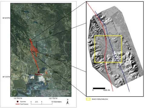
The city of Napa, California, USA is located within an area of major north-northwest-trending fault systems forming part of the greater San Andreas Fault system along the west coast of the United States. The closest active fault is the West Napa fault, a system of discontinuous strike-slip faults along the western margin of the geologic basin underlying Napa Valley. The Mw 6.0 24 August 2014 South Napa earthquake initiated 8km south-southwest of Napa and 1.7 km west of the West Napa fault system approximately 11.3 km below the surface (Brocher et al., 2015; Wei et al., 2015). The earthquake subsequently ruptured approximately 12 to 15 km in a northwest direction; the total rupture zone covering an area of approximately 75 km2. Only part of the rupture was connected to previously mapped portions of the West Napa system. Five surface rupture traces were field identified post-earthquake (Fig. 1). Moment tensors and focal mechanisms from the earthquake show fault slip along the fault system was that of a right-lateral strike slip earthquake, similar to movements seen throughout the region.
Figure 1. Map of field identified earthquake traces (red) in the Napa Valley after South Napa earthquake. Right inset shows DTM of the Browns Valley Neighborhood with buildings added. Yellow box shows area of detailed analysis for this study. Red line through
The earthquake displacements caused widespread infrastructure damage in Napa County and nearby Solano County with concentrated pockets of damage in areas such as the Browns Valley neighborhood, Cuttings Wharf, western and downtown Napa (Bray et al., 2014). For this study, we concentrated on the Browns Valley neighborhood in Napa (Fig. 1) to test and contrast the differential ALS change detection algorithms. Rates of fault slip in the Napa region before the earthquake varied between 1 and 9.5 mm/yr. along the West Napa fault (Barnhart et al., 2015; Brocher et al., 2015). Slip during the earthquake, or Coseismic slip, was measured to be between 1.5 and 46 cm along the earthquake rupture, with coseismic slip on the western trace of the study area measuring 23 cm in the south, decreasing to 6 cm further north and as high as 5 cm on the eastern trace (Brocher et al., 2015; Morelan et al., 2015). Slip post-earthquake, or afterslip, varied up and down the fault ranging from 10-20 cm per day in some locations to just over 40 mm in Browns Valley after 60 days (Hudnut et al., 2014). Cumulative displacement on the southern section of the western trace in the Browns Valley study area as of September 5th was measured to be approximately 34 cm by alignment array NLOD (Lienkaemper et al., 2016).
2. METHODS
2.1 ALS Datasets
The amount of displacement from the coseismic rupture was atypical for the magnitude of the Napa earthquake (Bray et al., 2014). The greater displacements allowed for visible offsets that could be measured by a wide array of survey instruments. Relevant to this study, the displacements were large enough to attempt estimation via the differencing of two ALS point clouds. Three different ALS datasets were acquired for this study (Table 1); two pre-earthquake datasets and one post-earthquake. The first pre-earthquake dataset was collected between May 15, 2003 and June 1, 2003 by the National Center for Airborne Laser Mapping (NCALM) in a study of the Napa River watershed from Calistoga, CA to San Pablo Bay. The instrument used was an Optech 2033 Airborne Laser Terrain Mapper (ALTM) with a resultant point density of 1.3 pts/m2. The second pre-earthquake dataset was collected June 7th, 2014 over Napa County, CA by Quantum Spatial as a mapping update for the city of Napa, CA. The instrument used in this collection flight was a Leica ALS60 with a nominal point density of 8 pts/m2. Following the earthquake rupture on August 24, 2014, a post-earthquake dataset was acquired by a consortium group for the express purpose of scanning the earthquake affected area in hopes of analysing the differential LiDAR results (Hudnut et al., 2014). An Optech Orion M300 scanner collecting point densities of ~11.4 pts/m2 was flown by Towill, Inc. on September 9, 2014. Both the 2003 dataset and September 2014 dataset are available for public access via opentopography.org (Hudnut et al., 2014). A short summary of ALS acquisition parameters from the three flights are included in Table 1 for comparison.
2.2 Change Detection Techniques
Differential LiDAR has proven exceptionally useful for documenting earthquake events, analysing their effects, and understanding earthquake mechanics (Hudnut et al. 2014; Nissen et al. 2012; Oskin et al. 2012; Brooks et al. 2014; Glennie et al. 2014; Zhang et al., 2015). There are many temporal spaced change detection methods for LiDAR point clouds including one dimensional slope based methods, two
dimensional image based methods, 2.5D digital elevation model (DEM) and mesh grid methods, and 3D point cloud methods (Zhang, 2016). This study focuses on a 2.5D method called Particle Image Velocimetry (PIV) and a 3D closest point based method called Iterative Control Point (ICP).
ICP is one of the most common change detection methods used on 3D point clouds. It is based on an algorithm that matches two point sets by iteratively minimizing the root mean squared distance (RMSD) between a target and reference 3D data set by rigidly transforming one data set to match the other until the change in RMSD between iterations reaches a pre-defined tolerance. Many versions of ICP exist, the standard ICP approach from Zhang et al., 2015, is used here. As seen in equation 1, we represent a point matching function as f and compute the RMSD between a 3D point cloud P and a reference 3D point cloud Q denoted by {pi}, i = 1 …Np and {qi}, i = 1 …Nq;
����(�,�,�) =�1
�∑��∈�‖��− �(��)‖2. (1)
The next objective is to minimize the RMSD. To do this, the point clouds are assumed to represent a rigid body and by applying a rigid transformation the point sets are moved to match each other. Using equation 2, a rigid transformation is estimated that minimizes the sum of the RMSD between the two point sets. In addition to equation 1 parameters, the rotation matrix is represented by R, the translation vectors by t, and
SO(d) represents special orthogonal matrices in d dimensions.
The process is iterated to find a global minimum. Because of the matching and transformation steps, the error or distance between point sets is monotonically reduced with the passing iterations (Zhang, 2016). Thusly, the entire process can be broken down into three primary steps; matching closest points, a rigid transformation of data sets, and the iteration of the first two steps until the change in the global RMSD statistic is minimized to a value below a pre-set threshold. If that minimum is reached, cumulative transformation rotations and translations represent the change over a temporal period between the two point sets. The algorithm is not fool proof though, often finding a local minimum instead of a global minimum due to data noise, outliers, low overlap, and poor data density. The original algorithm derivation can be found in Besl and McKay, 1992.
The ICP algorithm used for our study utilizes several variations from the original algorithm including uniform weighting and minimization, a moving window style point cloud selection to properly sample the entire data set for change, KD-tree searching for nearest neighbor style matching, as well as a geodetic marker technique explained in more detail below. The translations from each iteration are cumulated for all three dimensions and represent the total temporal displacements between the data sets. Results of each window sample in the ICP analysis are vectorised to illustrate the displacement field. All three datasets are inter-compared in batches of two; 2003 to June 2014, 2003 to September 2014, and June 2014 to September 2014.
The same dataset pairs are also analyzed using PIV, but this time only changes in the x and y direction can be displayed because PIV is a 2.5D method. PIV originated in the fluid mechanics field using pictures of a fluid flow and reflective particles in that fluid were analyzed with image to image matching to measure 2.5D change. The method has now advanced beyond those experiments to a modern digital image co-registration and correlation technique. As a sensitive change detection technique, it is effective in geotechnical studies using close range photography and with the growth of LiDAR has been used in the field to study deformation after earthquakes and from landslides (Aryal et al., 2015, 2012; Mukoyama, 2011). However, using 3D point clouds presents its own problems. To interpret the point clouds with PIV, the image plane becomes the horizontal x-y plane with the z-axis analogous to the light intensity of a traditional particle in PIV, hence the 2.5D designation (Aryal et al., 2012). From here, various steps of image pre and post processing can be applied, but the kernel of the algorithm in a common digital PIV method calculates the particle displacement by calculating the cross-correlation of many small sub-images taken from the study images to cumulatively yield the most probable displacement field between the two images. The cross correlation is applied with the direct cross correlation function (Eq. 3) that employs a statistical pattern matching technique to find the displacement pattern between a sub-image A and sub-image B. Original window indexes are represented by i and j with m and n representing displacement so that the location of the intensity peak in matrix C is the most probable displacement from A to B (Thielicke and Stamhuis, 2014).
C(m, n)= ∑ � ∑ �A(i, j)B�i-m, j-n� (3)
The PIV method applied here turned the 3D point clouds into 2D images via nearest neighbor interpolation of elevation to produce rasterized images. The PIV algorithm was applied with the Matlab toolbox PIVlab (Thielicke and Stamhuis, 2014). Pre-analysis image processing was carried out within the toolbox using Contrast Limited Adaptive Histogram Equalization (CLAHE), a Wiener denoising filter and highpass filter. During PIV evaluation, cross correlation was calculated in the frequency domain using fast fourier transforms (FFT). To reduce information loss, the images being compared were separately split up into iteratively smaller frames of 300, 100, and 20 pixel blocks from original 4401x4401 pixel images. In an iterative process to better interpret the displacements, the result of the correlation matrix from the first frames augmented the second iteration of frames using spline interpolation. This was repeated again for the third frame iteration. The peak of the correlation matrices was interpreted with a 2x3 Gaussian
function until there was a sum displacement vector for each 20 pixel image. The resulting data represented the displacement field of the earthquake. The final result of the PIV change detection was then vectorised for better illustration of the displacement field. Errors can occur using PIV due to user error, incorrect sizing of the image and sub-images, and small magnitude of the displacement (Aryal et al., 2012). Beyond those errors, the process should only introduce a bias smaller than 0.005 pixels and random noise below 0.02 pixels (Thielicke and Stamhuis, 2014). The pixel size in this study was 0.5 meters. Further documentation on the PIV algorithm can be found in Thielicke and Stamhuis, 2014, or at pivlab.blogspot.com.
Lastly, we attempted to include additional information in the point clouds to aid the change detection techniques used above. In previous differential LiDAR studies of earthquakes, change detection was performed with unaltered or bare earth point clouds representing only the ground so as to cut out vegetation and anthropogenic sources that cause noise in unaltered results (Nissen et al., 2012; Nissen et al., 2014; Zhang, 2016). In the same way, the Napa point clouds were classified using proprietary software packages and bare earth model point clouds were created. However, in addition to the bare earth returns, we created bare earth point clouds combined with manmade structures that we have termed geodetic markers. These easily identified objects are expected to be constant over the temporal gaps between point clouds and are analogous to the persistent scatterers of differential InSAR analyses where objects showing a strong, constant radar reflection over time are used to maintain phase coherence with InSAR (Crosetto et al., 2015; Ferretti et al., 2001). Persistent scattering has aided earthquake deformation measurements with InSAR and can be used in a mix of urban and natural environments (Crosetto et al., 2015; Kampes, 2006). Similarly, geodetic marker techniques for LiDAR point clouds have proven useful for point cloud change detection in urban environments (Kusari, 2015). Therefore, we used the roofs of structures in the point cloud as geodetic markers. The roofs are the most trustworthy sources for stable markers readily available to an ALS system’s viewpoint and due to the size of the earthquake indicate the earthquake displacement with any outliers representing possible structural damage. The same software packages used to retrieve bare earth points were used to retrieve and combine the geodetic markers with the bare earth points. Bare earth point clouds and point clouds enhanced with geodetic markers were then applied to both change detection algorithms.
3. RESULTS
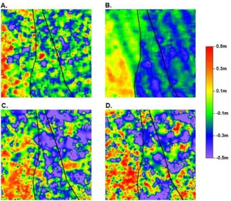
The ICP results using bare earth point clouds are shown in Figure 2A and 2B. The 2003 to 2014 differencing is largely incoherent with average right lateral displacement of 5 cm east of the western fault trace and standard deviations as high as 19 cm. However, the June to September 2014 differencing shows a clear delineation of the main fault segment from left to right.
The right lateral displacement from June to September has an average of 23.6 cm with a 7.4 cm standard deviation. The PIV results of the bare earth model show a very different result in Figures 2C and 2D. The 2003 to 2014 dataset is incoherent with only a slightly more discernible pattern in the June to September 2014 results. Average right lateral displacement is 18 cm for June to September and 24cm for 2003 to 2014. However, the standard deviations of the PIV results are far too large at 31 and 27 cm respectively.
A clear difference can be seen in the ICP results when including geodetic markers (Fig. 3), especially for the 2003 to 2014 differences. The average displacements and standard deviations of the ICP results have improved with the geodetic markers. All standard deviations are below twenty centimeters with the largest deviation from the 2003 to 2014 dataset at 19 cm on the western side of the fault. Average displacements on the eastern side are 15 cm for 2003 to 2014 and 23.5 cm for June to September (Fig. 4). Given the cumulative displacement of 34 cm at the bottom of the study area’s western trace, those results might be expected if the south to north decrease seen in the coseismic measurements is accounted for (Lienkaemper et al., 2016; Morelan et al., 2015). Furthermore, the displacement fields clearly show how landscape change over time by both natural and anthropogenic causes can mask the displacement when determined by ground surface alone. The June to September 2014 displacement for terrain only and terrain plus geodetic markers show mostly subtle variances but the 2003 to 2014 results show more obvious improvements with the inclusion of markers. In all cases, the variance of the resulting displacements is significantly improved using the geodetic markers.
The PIV results also showed some improvement when including geodetic markers to the point cloud. The June to September 2014 displacement field now shows a clear delineation of the fault trace and the displacement field shows far less noise. The June to September 2014 data shows average displacements with minimal displacement west of the fault and an average displacement of 39cm to the east, above the expected displacement compared to field measurements. Standard deviation is less now, with results east of the fault returning an acceptable 20 cm of deviation and west of the fault 26 cm. However, the 2003 to 2014 results showed little to no improvement with an average displacement of 13 cm east of the fault and enduring noise having the deviation in the east decrease to 24 cm but western deviation increase to 30 cm.
The statistics of the results, and their trends, can be seen in the box plots of figure 4. The maximum and minimum values along with the boxes reflecting the interquartile range (IQR) show the distribution of the results and reflect their noise. A pattern characteristic of right lateral displacements can be seen where results west of the main rupture are minimal, centered near zero displacement. Additionally, the statistics allow us to draw further conclusions when comparing the two algorithms. ICP consistently has lower ranges and smaller IQRs. Lastly, the effect of longer temporal spacing can also be seen in the box plots. The ICP and PIV results for June to September 2014, especially east of the fault, have smaller IQR and median values are closer to the measured displacements in the Browns Valley study area.
Figure 2. Displacement fields in the Y direction from bare earth point clouds. Fault traces shown by black lines. (A) ICP results of
differenced point clouds from 2003 to September 2014. (B) ICP results of differenced point clouds from June 2014 to September 2014. (C) PIV results of differenced point clouds from 2003 to September 2014. (D) PIV results of differenced point clouds from
June 2014 to September 2014.
Figure 3. Displacement fields in the Y direction from geodetic marker point clouds. Fault traces shown by black lines. (A) ICP
results of differenced point clouds from 2003 to September 2014. (B) ICP results of differenced point clouds from June 2014 to September 2014. (C) PIV results of differenced point
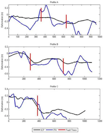
An analysis of Figure 5 shows interesting patterns in the profiles from both algorithms. Profiles B and C show distinct increase in absolute displacement, or slope change, as the profiles cross the fault traces. In large part, the changes at the west trace go from near zero west of the trace to near 30 cm of displacement east of trace, which we might expect given the surveys of slip along that rupture (Hudnut et al., 2014). As a whole though, the profiles show the distinct difference in results between the algorithms. The PIV results (as confirmed in Figure 4) have much more noise, exemplified by the many peaks and
valleys across the profiles, whereas the ICP results are much smoother and seemingly more reliable. Further work could use these types of profiles to better understand the spatial distribution of slip in the near field for geophysical models as well as determine whether the irregular PIV profile or smooth ICP profile better fits the distribution of slip near the fault.
4. CONCLUSION
Both change detection algorithms provided discernible results with varying levels of accuracy and adherence to the known displacement fields of the earthquake. Therefore, in conclusion, both change detection techniques are able to recover near field deformation where other geodetic techniques do not. The faults were clearly delineated in all but four results with average right lateral displacement estimates for all applications ranging between 5 and 39 cm. Compared to the coseismic and cumulative displacements listed above, these results cover that entire range from 5 to 34 cm in the study area especially considering spatial differences in measurement sites and assumed noise. Patterns in figures 2 and 3 as well as the average displacements also mirror the general decrease in displacement moving north along the western fault trace.
Standard deviations of the best results were at or below an accepted ALS horizontal resolution limit of 20 cm. The ICP method returns the lowest standard deviations, most improvement between temporal gaps and as can be seen in figures 2 to 5, displacement fields with the least amount of noise and generally the most reliable results with best agreement to the independent survey measurements. PIV provides distinctive displacement fields and interesting results but the amount of error and noise is considerably higher. Reflecting on these results, it is clear that ICP is likely the best change detection algorithm for ALS near-field deformation estimation.
The analysis also presents obvious evidence of degradation in estimation accuracy with increased temporal separation between the two point clouds. The smaller time gap provided more consistent results with a standard deviation on average 5cm better. This is partially due to the noise built up from natural variations in the point cloud, whether anthropogenic or natural. Figure 4. Box plots of ICP results and PIV results from geodetic marker point clouds, separated by points east and west of the
main western fault trace over two temporal periods, 2003 to September 2014 and June 2014 to September 2014.
However, not all of this degradation is due to the time spacing between datasets; the most likely cause of the improvement is improved instrumentation and better survey parameters (i.e. point density) for the 2014 ALS acquisitions.
Finally, the inclusion of the geodetic markers was shown to improve the results from both change detection algorithms. ICP showed improvement as a whole as well as noticeable improvement for the large temporal spacing datasets while PIV showed marginal improvement for one of the comparison datasets. This suggests that the geodetic markers help mitigate problems due to the point density fall off between old and new systems for large temporal gap analyses when conducting ICP. However, the lack of considerable improvement using geodetic markers with PIV is counter-intuitive considering how particles typically found in PIV methods are akin to geodetic markers. One possibility to improve PIV results may be to pay more attention to the pre-processing of the PIV images. The improved coherence from geodetic markers may be negated by the effects of pre-process sampling and filtering of the input images. Regardless, there is clear evidence that the geodetic marker results encourage the use of some classified point clouds in differential LiDAR analyses instead of bare earth or unaltered clouds. Our future work will continue analysing the PIV application for differential LiDAR as well as continue to experiment with other change detection methods. We also plan to expand the analysis to larger study sites in the Napa Valley. This will hopefully provide input observations for geophysical inversion models of the Napa earthquake.
ACKNOWLEDGEMENTS
Partial support for the analysis of displacement was provided by the USGS through a cooperative agreement with the University of Houston.
REFERENCES
Aryal, A., Brooks, B.A., Reid, M.E., 2015. Landslide subsurface slip geometry inferred from 3-D surface displacement fields. Geophys. Res. Lett. 42, 1411-1417.
Aryal, A., Brooks, B.A., Reid, M.E., Bawden, G.W., Pawlak, G.R., 2012. Displacement fields from point cloud data: Application of particle imaging velocimetry to landslide geodesy. J. Geophys. Res. Earth Surf. 117, F01029.
Barnhart, W.D., Murray, J.R., Yun, S.-H., Svarc, J.L., Samsonov, S.V., Fielding, E.J., Brooks, B.A., Milillo, P., 2015. Geodetic Constraints on the 2014 M 6.0 South Napa Earthquake. Seismol. Res. Lett. 86, 335–343.
Besl, P.J., McKay, N.D., 1992. A method for registration of 3-D shapes. IEEE Trans. Pattern Anal. Mach. Intell. 14, 239–256.
Bray, J., Cohen-Waeber, J., Dawson, T., Kishida, T., Sitar, N., 2014. Geotechnical engineering reconnaissance of the August 24, 2014 M 6 South Napa earthquake. Geotech. Extreme Events
Reconnaiss. GEER Assoc. Rep. Number GEER 37.
Brocher, T.M., Baltay, A.S., Hardebeck, J.L., Pollitz, F.F., Murray, J.R., Llenos, A.L., Schwartz, D.P., Blair, J.L., Ponti, D.J., Lienkaemper, J.J., Langenheim, V.E., Dawson, T.E., Hudnut, K.W., Shelly, D.R., Dreger, D.S., Boatwright, J., Aagaard, B.T., Wald, D.J., Allen, R.M., Barnhart, W.D., Knudsen, K.L., Brooks, B.A., Scharer, K.M., 2015. The Mw 6.0
24 August 2014 South Napa Earthquake. Seismol. Res. Lett. 86, 309–326.
Brooks, B.A., Hudnut, K.W., Glennie, C.L., Ericksen, T., 2014. Near-Field Deformation Associated with the M6.0 South Napa Earthquake Surface Rupture. AGU Fall Meet. Abstr. S33F-4900.
Crosetto, M., Monserrat, O., Cuevas-González, M., Devanthéry, N., Crippa, B., 2015. Persistent Scatterer Interferometry: A review. ISPRS J. Photogramm. Remote Sens.
Ferretti, A., Prati, C., Rocca, F., 2001. Permanent scatterers in SAR interferometry. IEEE Trans. Geosci. Remote Sens. 39, 8– 20.
Glennie, C.L., Carter, W.E., Shrestha, R.L., Dietrich, W.E., 2013. Geodetic imaging with airborne LiDAR: the Earth’s surface revealed. Rep. Prog. Phys. 76, 086801.
Glennie, C.L., Hinojosa-Corona, A., Nissen, E., Kusari, A., Oskin, M.E., Arrowsmith, J.R., Borsa, A., 2014. Optimization of legacy lidar data sets for measuring near-field earthquake displacements. Geophys. Res. Lett. 41, 3494-3501.
Hudnut, K.W., Brocher, T.M., Prentice, C.S., Boatwright, J., Brooks, B.A., Aagaard, B.T., Blair, J.L., Fletcher, J., Erdem, J.E., Wicks, C.W., others, 2014. Key recovery factors for the August 24, 2014, South Napa earthquake. US Geol Surv
Open-File Rept 1249, 51.
Kampes, B.M., 2006. Radar Interferometry: Persistent Scatterer Technique, Remote Sensing and Digital Image Processing.
Springer Netherlands.
Kusari, A., 2015. Precise Registration of Laser Mapping Data by Planar Feature Extraction for Deformation Mapping (Ph.D. Dissertation). University of Houston, Houston, TX.
Lienkaemper, J.J., Brooks, B.A., DeLong, S.B., Domrose, C.J., Rosa, C.M., 2014. Surface slip associated with the 2014 South Napa, California earthquake measured on alinement arrays.
AGU Fall Meet. Abstr. S33F-4898
Lienkaemper, J.J., DeLong, S.B., Domrose, C.J., Rosa, C.M., 2016. Afterslip Behavior following the 2014 M 6.0 South Napa Earthquake with Implications for Afterslip Forecasting on Other Seismogenic Faults. Seismol. Res. Lett.
Morelan, A.E., Trexler, C.C., Oskin, M.E., 2015. Surface‐
Rupture and Slip Observations on the Day of the 24 August 2014 South Napa Earthquake. Seismol. Res. Lett. 86, 1119– 1127.
Mukoyama, S., 2011. Estimation of ground deformation caused by the earthquake (M7.2) in Japan, 2008, from the geomorphic image analysis of high resolution LiDAR DEMs. J. Mt. Sci. 8, 239–245.
Nissen, E., Krishnan, A.K., Arrowsmith, J.R., Saripalli, S., 2012. Three-dimensional surface displacements and rotations from differencing pre- and post-earthquake LiDAR point clouds. Geophys. Res. Lett. 39, L16301.
Nissen, E., Maruyama, T., Ramon Arrowsmith, J., Elliott, J.R., Krishnan, A.K., Oskin, M.E., Saripalli, S., 2014. Coseismic fault zone deformation revealed with differential lidar: Examples from Japanese ∼7 intraplate earthquakes. Earth
Oskin, M.E., Arrowsmith, J.R., Corona, A.H., Elliott, A.J., Fletcher, J.M., Fielding, E.J., Gold, P.O., Garcia, J.J.G., Hudnut, K.W., Liu-Zeng, J., Teran, O.J., 2012. Near-Field Deformation from the El Mayor–Cucapah Earthquake Revealed by Differential LIDAR. Science 335, 702–705.
Rice, J.R., Cocco, M., 2007. Seismic fault rheology and earthquake dynamics. Tecton. Faults Agents Change Dyn. Earth 99–137.
Thielicke, W., Stamhuis, E.J., 2014. PIVlab – Towards User-friendly, Affordable and Accurate Digital Particle Image Velocimetry in MATLAB. J. Open Res. Softw. 2(1).
Wei, S., Barbot, S., Graves, R., Lienkaemper, J.J., Wang, T., Hudnut, K., Fu, Y., Helmberger, D., 2015. The 2014 Mw 6.1 South Napa Earthquake: A Unilateral Rupture with Shallow Asperity and Rapid Afterslip. Seismol. Res. Lett. 86, 344–354.
Zhang, X., 2016. LiDAR Based Change Detection for Earthquake Surface Ruptures (Ph.D. Dissertation). University of Houston, Houston, TX.
Zhang, X., Glennie, C., Kusari, A., 2015. Change Detection From Differential Airborne LiDAR Using a Weighted Anisotropic Iterative Closest Point Algorithm. IEEE J. Sel. Top.