MAPPING LAND COVER IN THE TAITA HILLS, SE KENYA, USING AIRBORNE
LASER SCANNING AND IMAGING SPECTROSCOPY DATA FUSION
R. Piiroinen a,1*, J. Heiskanen a, E. Maeda a, P. Hurskainen a, J. Hietanen a, P. Pellikka a
a Department of Geosciences and Geography, P. O. Box 64, FI-00014 University of Helsinki, Finland – (rami.piiroinen,
janne.heiskanen, eduardo.maeda, pekka.hurskainen, jesse.hietanen, petri.pellikka)@helsinki.fi.
KEY WORDS: GEOBIA, LCCS, Hyperspectral data, LiDAR, Data fusion, Object-based classification
ABSTRACT:
The Taita Hills, located in south-eastern Kenya, is one of the world’s biodiversity hotspots. Despite the recognized ecological importance of this region, the landscape has been heavily fragmented due to hundreds of years of human activity. Most of the natural vegetation has been converted for agroforestry, croplands and exotic forest plantations, resulting in a very heterogeneous landscape. Given this complex agro-ecological context, characterizing land cover using traditional remote sensing methods is extremely challenging. The objective of this study was to map land cover in a selected area of the Taita Hills using data fusion of airborne laser scanning (ALS) and imaging spectroscopy (IS) data. Land Cover Classification System (LCCS) was used to derive land cover nomenclature, while the height and percentage cover classifiers were used to create objective definitions for the classes. Simultaneous ALS and IS data were acquired over a 10 km × 10 km area in February 2013 of which 1 km × 8 km test site was selected. The ALS data had mean pulse density of 9.6 pulses/m2, while the IS data had spatial resolution of 1 m and spectral resolution of 4.5–5 nm in the 400–1000 nm spectral range. Both IS and ALS data were geometrically co-registered and IS data processed to at-surface reflectance. While IS data is suitable for determining land cover types based on their spectral properties, the advantage of ALS data is the derivation of vegetation structural parameters, such as tree height and crown cover, which are crucial in the LCCS nomenclature. Geographic object-based image analysis (GEOBIA) was used for segmentation and classification at two scales. The benefits of GEOBIA and ALS/IS data fusion for characterizing heterogeneous landscape were assessed, and ALS and IS data were considered complementary. GEOBIA was found useful in implementing the LCCS based classification, which would be difficult to map using pixel-based methods.
*Corresponding author
1. INTRODUCTION
The land cover has changed rapidly in the Taita Hills, in south-eastern Kenya. Large areas of forests, woodlands and shrublands have been converted into agricultural use (Clark and Pellikka, 2009; Pellikka et al., 2009). However, mapping these changes using remote sensing (RS) is a challenging task as even the class definitions are based on heuristic views of given classification system. The land cover in the area is very heterogeneous and consists mostly of mixed classes of trees, crops and other vegetation.
Mapping heterogeneous classes using L-resolution satellite data is difficult, since individual components (e.g. single trees) that form agroforestry or woodland classes cannot be distinguished (Zomer et al. 2009; Blinn et al. 2013). On the other hand, using H-resolution data allows a clear distinction of individual trees (e.g. Eysn et al., 2012; Dalponte et al., 2014). However, linking individual trees to certain minimum mapping unit (MMU) of agricultural land, which would represent agroforestry is challenging (Zomer et al., 2009; Blinn et al., 2013). L-resolution data refers to situations where the scene objects are smaller than the pixel size of the data, while in H-resolution data the scene objects are larger than the pixel size (Strahler et al., 1986).
Mapping mixed land cover classes accurately is important because agroforestry has high potential for carbon sequestration in developing countries (Negash and Kanninen, 2015).
Agroforestry could be a direct target in REDD+ programs depending on the country’s forest definition (Minang et al., 2014). In REDD+ programs the countries are rewarded for keeping forests and reducing emissions from deforestation. Agroforestry is, however, not been mentioned in REDD+ programs, despite its proven climate change mitigation and adaptation benefits (Minang et al., 2014). Trees outside forests (TOF) also have importance on local and regional scale economy. For example, in India TOFs constitute estimated 49 % of the annual fuelwood and 48% of the annual timber consumed (Panday, 2002).
the fractions of finer scale land cover types (e.g. crops and trees) they contain.
Furthermore, combining optical data with Light Detection and Ranging (LiDAR) technology could highly improve the accuracy of land cover classification in agroforestry areas. Unfortunately, this approach has not yet been fully explored, in particular in tropical mountain environments.
In this article, H-resolution airborne laser scanning (ALS) and imaging spectroscopy (IS) data fusion (Torabzadeh et al., 2014) was used together with GEOBIA to characterize the mixed land cover classes based on biophysical definitions derived from Land Cover Classification System (LCCS) (Di Gregorio, 2005). ALS enables the use of accurate three dimensional information of the land cover, while IS enables the detection of different materials based on their spectral characteristics. In this study our objectives were to:
(i) create clear definitions for the land cover classes based on LCCS and measurable biophysical attributes (tree height, crown cover) that are non-overlapping and measurable using remote sensing methods.
(ii) test multiscale segmentation for defining mapping units for characterizing heterogeneous landscape with emphasis on forests and agroforestry.
(iii) assess the benefits of data fusion in creating the land cover classes.
2. MATERIAL
2.1 Study area
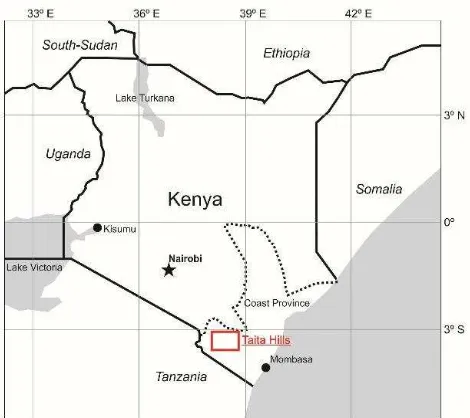
The study area (8 km × 1 km) is located in the elevation range of 1100–1800 m a.s.l. in the highlands of the Taita Hills (3° 25′ S, 38° 19′ E) in south-eastern Kenya (Figure 1). There are two rainy seasons with long rains occurring in the March-June and short rains in October-December (Jaetzold and Schmidt, 1983).
Figure 1. Location of the Taita Hills in south-eastern Kenya.
2.2 Airborne data collection
Flight campaign was conducted in 3–8.2.2013 during the dry season. Two sensors were used to collect ALS and IS data from mean flying height of 750 m. Optech ALTM 3100 (Optech, Canada) is an oscillating mirror laser scanner capable of recording up to four echoes. The sensor was operated with pulse rate of 100 kHz and scan rate of 36 Hz. Scan angle was ±16°. Achieved pulse density was 9.6 pulses m−2. Mean footprint diameter was 23 cm. AisaEAGLE is a pushbroom scanner with instantaneous field of view of 0.648 mrad and field of view of 36.04° (Spectral Imaging Ltd., Finland). The sensor was used in four times spectral binning mode that produces output images with 129 bands and full width at half maximum of 4.5–5.0 nm in spectral range of 400–1000 nm. The output pixel size was 1.0 meters.
3. METHODS
3.1 Preprocessing of the data
ALS data was pre-processed by the data vendor (Topscan Gmbh) and delivered as a georeferenced point cloud in UTM/WGS84 coordinate system with ellipsoidal heights. TerraScan software (Terrasolid Ltd., Finland) was used to create digital terrain model (DTM) and digital surface model (DSM) from ALS data, which was classified to ground and other returns. Some of the very steep slopes were falsely classified and had to be manually corrected. The first returns were used to create DSM and the returns classified as ground to create DTM at 1 m resolution. DTM values were subtracted from DSM values to create canopy height model (CHM), which represents the height of vegetation and buildings from the ground level (CHMbuildings). Another CHM was created using the same approach, but the power lines were first removed manually and returns classified as buildings were removed (CHMnobuildings). DTM was used for calculating slope.
The raw data produced by AisaEAGLE was radiometrically corrected and georectified with CaliGeoPro 2.2 (Spectral Imaging Ltd., Finland). DSM derived from ALS data was interpolated to pixel size of 3 meters and used in the georectification process. Atmospheric correction was applied using ATCOR-4 (Schläpfer and Richter, 2002).
After the initial georectification of AisaEAGLE data, it was noted that there were geometric mismatches between AisaEAGLE and ALS data. The geometric accuracy of the ALS data was assumed to be better and thus CHMbuildings was used as a reference data for manual co-registration of AisaEAGLE data. The processed flight lines were first subsetted so that the side overlap between images was minimized. Next, 50–100 control points were collected from CHMbuildings and AisaEAGLE data for each flight line. Then, the first order polynomial transformation was applied to co-register the AisaEAGLE flight lines and CHMbuildings. After co-registration, RMSE for an example flight line was 1.06 pixels (meters), which was considered accurate enough for data fusion (Valbuena, 2014).
3.2 LCCS class definitions
clear physiognomic aspects of a tree. Mapping physiognomic aspects using RS is challenging and thus all the plants taller than 3 m were considered as trees. Forest is defined typically based on certain tree crown cover (CC) on MMU (Magdon and Klein, 2013; Eysn et al., 2013). CC refers to the proportion of the forest floor covered by the vertical projection of the tree crowns (Jennings et al., 1999; Korhonen et al., 2006). For example, UNFCCC as part of Kyoto protocol states that: ‘forest is a minimum area of land of 0.05-1.0 hectares with tree crown cover (or equivalent stocking level) of more than 10-30 per cent with trees with the potential to reach a minimum height of 2-5 metres at maturity in situ’ (Minang et al., 2014). FAO uses 10 % CC threshold and 0.5 ha MMU (FAO, 2000). LCCS does not define a specific MMU for forests or any other land cover type.
ICRAF (1993) defines agroforestry as follows: “Agroforestry is a collective name for land-use systems and technologies, where woody perennials are deliberately used on the same land management unit as agricultural crops and/or animals, either in some form of spatial arrangement or temporal sequence. In agroforestry systems there are both ecological and economical interactions between the different components”. Panday (2002) defines it to include all forms of tree-growing in agroecosystems. Mapping agroforestry is difficult using RS methods and thus in this article agroforestry refers to trees on farmland. The CC thresholds for defining the agroforestry and woodland classes were derived from LCCS percentage cover classifier.
3.3 Segmentation and classification
Segmentation and classification was done in eCognition Developer (Trimble Navigation, Ltd.). First, multiresolution segmentation (MRS) was used to create level-0 segmentation based on normalized difference vegetation index (NDVI; Tucker, 1979) and CHM using scale parameter of 275, shape of 0.5 and compactness of 0.7. Next, MRS was used for level-1 segmentation inside level-0 segments based on CHM using scale parameter of 25, shape of 0.2 and compactness of 0.6.
The classification was done first on level-1. The first step was to separate all trees. This was done based on CHMnobuildings where all targets taller than 3 m were classified as trees. Next, CHMbuildings was used to classify the remaining targets that were taller than 3 m as buildings. A temporary class was created for objects with heights between 1–3 m and training samples were collected for buildings and shrubs. Training samples were collected visually using AisaEAGLE data. Support Vector Machine (SVM) classification (Vapnik, 1998; Mountrakis et al., 2011) was applied using 12 first minimum noise fraction (MNF) transformed (Green et al., 1988) AisaEAGLE bands to classify all 1–3 m objects into buildings and shrubs. 12 MNF bands have been shown to yield highest classification accuracies with AisaEAGLE data in a previous study (Piiroinen et al., 2015).
The remaining objects were classified into a temporary class and merged to create one segment containing all objects of 0–1 m height. This object was segmented based only on NDVI for better separation of bare soil, water and low vegetation targets. SVM classification was applied using median NDVI as input to separate these classes. Level-0 classification was based on level-1 classes and LCCS class definitions.
4. RESULTS AND DISCUSSION
4.1 LCCS class definitions and their implementation based on GEOBIA approach
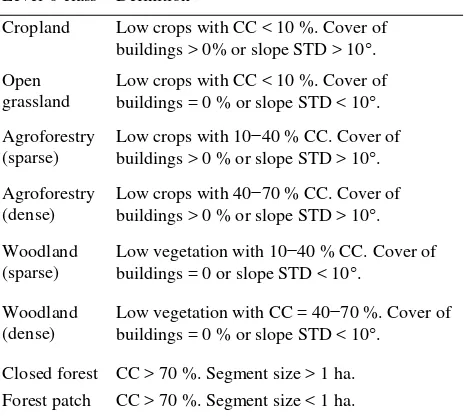
We created eight level-0 classes based on LCCS (Table 1). These classes were composed of finer scale segmentation and classification results based on six land cover classes described in Table 2. As agricultural land and other low vegetation targets were not separated at level-1, the presence of buildings was used as criteria to separate agroforestry and woodland classes. This approach is based on the knowledge that in the study area agriculture is practiced mainly on small scale family farms, in which cultivated areas are located next to buildings. One of the strengths of GEOBIA approach is to take advantage of these context based rules to separate classes that are hard to separate based only on their biophysical characteristics (Blaschke et al., 2014).
Further visual analysis showed that remaining agroforestry and agricultural land, without nearby buildings, were still present in the level-0 segments. These remaining agricultural areas were separated based on the presence of terraces. Agricultural terraces were detected based on the standard deviation (STD) of the terrain slope, given that terraced farms are combinations of very steep slopes and levelled terraces, which makes the STD implicitly. Agroforestry would belong to cultivated and managed lands, while cover and height classifiers are included only for natural and semi-natural terrestrial class. This prevents using LCCS as such to characterize agroforestry systems and further interpretations of the system are left for the user.
ALS data makes it possible to use LCCS height classifier in land cover characterization, which makes it possible to use unambiguous and objective threshold values for trees, shrubs and low vegetation. Percentage cover classifier can be used to define mixed land cover classes. However, there is very little discussion in the LCCS manual on how the MMUs should be selected, while this is a key element in forming the classes.
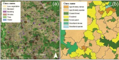
Level-0 class Definition
Cropland Low crops with CC < 10 %. Cover of buildings > 0% or slope STD > 10.
Open grassland
Low crops with CC < 10 %. Cover of buildings = 0 % or slope STD < 10.
Agroforestry (sparse)
Low crops with 10−40 % CC. Cover of buildings > 0 % or slope STD > 10.
Agroforestry (dense)
Low crops with 40−70 % CC. Cover of buildings > 0 % or slope STD > 10.
Woodland (sparse)
Low vegetation with 10−40 % CC. Cover of buildings = 0 or slope STD < 10.
Woodland (dense)
Low vegetation with CC = 40−70 %. Cover of buildings = 0 % or slope STD < 10.
Closed forest CC > 70 %. Segment size > 1 ha. Forest patch CC > 70 %. Segment size < 1 ha.
Table 1. Land cover classes based on LCCS at level-0.
Level-1 class Definition
Tree Vegetation with height > 3 m.
Building Built-up area with height > 3 m. Buildings 1-3 m classified with SVM based on 12 first MNF transformed AisaEAGLE bands.
Water Height < 1 m. Classified with SVM based on median NDVI.
Low vegetation
Height < 1 m. Classified with SVM based on median NDVI.
Shrub Vegetation with height 1-3 m. Classified with SVM based on 12 first MNF transformed AisaEAGLE bands.
Bare soil Height < 1 m. Classified with SVM based on median NDVI.
Table 2. Land cover classes at level-1.
4.2 Data fusion and multi-scale segmentation results
CHMbuildings shows the height of targets above ground (Figure 2a) while IS data shows the reflectance (Figure 2b). The results of the level-0 segmentation based on NDVI and CHM are presented in Figure 2c. The shape value was set to 0.5 so that the segments would include heterogeneous objects of trees and low vegetation while the forest patches with sharp edges were still separated into their own segments. Both data sources were shown to be important for creating meaningful segments, as segments based only on CHM would stick too closely to individual trees. NDVI was used instead of reflectance to minimize the influence of shadows. The level-1 segmentation, which was based only on CHM and smaller scale parameter separated trees and buildings in their own segments (Figure 2d).
Figure 2. Examples of canopy height model (a), AISA data (b), level-0 segmentation (c) and level-1 segmentation inside level-0
segments (d).
Our results show that in highly heterogeneous landscapes, the fusion of ALS and optical data was essential for successful separation of targets that could not be distinguished independently by using either ALS or IS data. For instance, ALS data created segments that followed trees and buildings very closely (Figure 3a), while it could not separate bare soil from low vegetation (Figure 3b).
Figure 3. Segmentation based on CHM (a) creates segments based on their height and thus it does not differentiate between
very low vegetation and bare soil. NDVI based segmentation separates the bare soil from the very low vegetation (b).
The classification based on level-1 segmentation was successful in separating the main land cover components (Figure 4a). However, this evaluation is based on visual interpretation and further validation is needed for a more comprehensive accuracy assessment. The validation will be possible when the classification is extended to the complete study area of 10 km × 10 km where field data collected in 2012, 2013 and 2014 are available.
Figure 4. Example of the level-1 classification (a) and level-0 classification based on the fractional cover of level-1 classes
(b).
The benefits of data fusion in segmentation and classification process were evident as, for example, CHM was very suitable for segmenting and classifying trees, while AisaEAGLE data was suitable for segmenting and classifying bare soil, water and low vegetation. These results are in agreement with Torabzadeh et al. (2014), who concluded that, at the moment, land cover maps are RS products that are benefiting the most from ALS and IS data fusion.
5. CONCLUSIONS AND FURTHER DEVELOPMENTS
LCCS was successfully modified to characterize mixed land cover classes like agroforestry. The height and percentage cover classifiers are useful when these classes are defined as objectively as possible. Multiresolution segmentation and multiscale approach created meaningful mapping units for the classes, while further validation of the results is needed before making more detailed conclusions. The benefit of this approach over pixel based methods is that clear threshold values can be used when the classes are defined and mapped. ALS and IS data nicely complemented each other, while all the potential of IS data was not used at this stage. The importance of IS increases as the classification is extended to species level. Species level information can then be used for more detailed definitions of level-0 classes. Information of tree types is important for agroforestry classification as farmers are known to plant specific species on their farmland for specific purposes. The strength of GEOBIA approach is to include these context based rules in the classification process. Future efforts will extend the classification system to our entire study area and the results will be validated based on field surveys. These results, together with further assessments of above ground biomass, will be used for assessing the carbon stocks and biodiversity in different land cover classes. This information will be highly beneficial for researchers and policy makers aiming to promote agroforestry practices and the design of biodiversity conservation plans.
ACKNOWLEDGEMENTS
The airborne remote sensing campaigns were funded by two projects from the Ministry for Foreign Affairs of Finland, namely by CHIESA (Climate Change Impacts on Ecosystem Services and Food Security in Eastern Africa) and BIODEV (Building Biocarbon and Rural Development in West Africa. Petri Pellikka is the Principal Investigator of both projects. Dr. Heiskanen and Mr. Jesse Hietanen work in BIODEV, Mr. Hurskainen and Mr. Piiroinen work in CHIESA, while Dr. Maeda is currently funded by a research grant from the Academy of Finland. The authors would also like to acknowledge the Taita Research Station of the University of
Helsinki in Kenya for the logistical support. We wish to thank Elisa Schäfer, Arto Viinikka and Hari Adhikari for their efforts in producing high quality georectification for AisaEAGLE data and co-registration of the two data products used.
REFERENCES
Arvor, D., Durieux, L., Andrés, S., Laporte, M.-A., 2013. Advances in geographic object-based image analysis with ontologies: a review of main contributions and limitations from a remote sensing perspective. ISPRS Journal of Photogrammetry and Remote Sensing, 82, pp. 125-137.
Belgiu, M., Dragut, L., 2014. Comparing supervised and unsupervised multiresolution segmentation approaches for extracting buildings from very high resolution imagery. ISPRS Journal of Photogrammetry and Remote Sensing, 96, pp. 67-75.
Benz, U.C., Hofmann, P., Willhauck, G., Lingenfelder, I. Heynen, M., 2004. Multi-resolution, object-oriented fuzzy analysis of remote sensing data for GIS-ready information.
ISPRS Journal of Photogrammetry & Remote Sensing, 58, pp. 239-258.
Bisseleua, D.H.B., Missoup, A.D., Vidal, S., 2009. Biodiversity conservation, ecosystem functioning and economic incentives under cocoa agroforestry intensification. Conservation Biology, 23(5), pp. 1176-1184.
Blaschke, T., Hay, G.J., Kelly, M., Lang, S., Hofmann, P., Addink, E., Feitosa, R.Q., van der Meer, F., van der Werff, H., van Coillie, F., Tiede, D., 2014. Geographic object-based image analysis – Towards a new paradigm. ISPRS Journal of Photogrammetry and Remote Sensing, 87, pp. 180-191.
Blinn, C.E., Browder, J. O., Pedlowski, M. A., Wynne, R. H., 2013. Rebuilding the Brazilian rainforest: Agroforestry strategies for secondary forest succession. Applied Geography, 43, pp. 171-181.
Clark, B.J.F., Pellikka, P.K., 2009. Landscape analysis using multi-scale segmentation and object-oriented classification. In: Röder, A., Hill, J. (Eds.), Recent Advances in Remote Sensing and Geoinformation Processing for land Degradation Assessment, pp. 323-342. Taylor & Francis Group, London.
Dalponte, M., Ørka, H.O., Ene, L.T., Gobakken, T. Næsset, E., 2014. Tree crown delineation and tree species classification in boreal forests using hyperspectral and ALS data. Remote Sensing of Environment, 140, pp. 306-317.
Di Gregorio, A. 2005. Land cover classification system – Classification concepts and user manual – Software version 2. Food and Agriculture Organization of the United Nations, Rome. pp. 190.
Eysn, L., Hollaus, M., Schadauer, K., Pfeifer, N., 2012. Forest delineation based on airborne LIDAR data. Remote Sensing, 4, pp. 762-783.
FAO, 2000. FRA 2000 – On definitions of forest and forest change. Food and Agriculture Organization of the United Nations – Forestry Department. Working Paper 33, Rome 2000.
quality with implications for noise removal. IEEE Transactions on Geoscience and Remote Sensing, 26(1), pp. 65-74.
Hay, G.J., Castilla, G., Wulderr, M.A., Ruiz, J.R., 2005. An automated object-based approach for the multiscale image segmentation of forest scenes. International Journal of Applied Earth Observation and Geoinformation, 7, pp. 339-359.
ICRAF, 1993. Annual report 1993. International Centre for Research in Agroforestry. Nairobi, Kenya. pp 208.
Jaetzold, R., Schmidt, H., 1983. Farm management handbook of Kenya. Natural conditions and farm management information 2 C. Ministry of Agriculture, Kenya & German Agricultural Team, German Agency for Technical Cooperation. Rossdorf, Germany.
Jennings, S. B., Brown, N. D., Sheil, D., 1999. Assessing forest canopies and understorey illumination: canopy closure, canopy cover and other measures. Forestry 72(1), pp. 59-74.
Korhonen, L., Korhonen, K. T., Rautiainen, M., Stenberg, P., 2006. Estimation of forest canopy cover: a comparison of field measurement techniques. Silva Fennica, 40(4), pp. 577-588.
Magdon, P., Kleinn, C., 2013. Uncertainties of forest area estimates caused by the minimum crown cover criterion.
Environmental Monitoring and Assessment, 185, pp. 5345-5360.
Minang, P.A., Duguma, L.A., Bernard, F., Mertz, O., van Noordwijk, M., 2014. Current Opinion in Environmental Sustainability, 6, pp. 78-82.
Mountrakis, G., Im, J., Ogole, C., 2011. Support vector machines in remote sensing: a review. ISPRS Journal of Photogrammetry and Remote Sensing, 66, 247-259.
Negash, M., Kanninen, M. 2015. Modeling biomass and soil carbon sequestration of indigenous agroforestry systems using CO2FIX approach. Agriculture, Ecosystems and Environment, 203, pp. 147-155.
Panday, D.N., 2002. Carbon sequestration in agroforestry systems. Climate policy, 2, pp. 367-377.
Pellikka, P., Lötjönen, M., Siljander, M., Lens, L., 2009. Airborne remote sensing of spatiotemporal change (1955–2004) in indigenous and exotic forest cover in the Taita Hills, Kenya. International Journal of Applied Earth Observation and Geoinformation, 11, pp. 221-232.
Piiroinen, R., Heiskanen, J., Mõttus, M., Pellikka, P., 2015. Classification of crops across heterogeneous agricultural landscape in Kenya using AisaEAGLE imaging spectroscopy data. International Journal of Applied Earth Observation and Geoinformation, 39, pp. 1-8.
Schläpfer, D., Richter, R., 2002. Geo-atmospheric processing of airborne imaging spectroscopy data. Part 1: parametric orthorectification. International Journal of Remote Sensing, 23(13), pp. 2609-2630.
Strahler, A-H., Woodcock, C.E., Smith, J.A., 1986. On the nature of models in remote sensing. Remote Sensing of Environment, 20, pp. 121-139.
Torabzadeh, H., Morsdorf, F., Schaepman, M.E., 2014. Fusion of imaging spectroscopy and airborne laser scanning data for characterization of forest ecosystems – A review. ISPRS Journal of Photogrammetry and Remote Sensing, 97, pp. 25-35.
Valbuena, R., 2014. Integrating airborne laser scanning with data from global navigation satellite systems and optical sensors. In: Maltamo, M., Næsset, E. and Vauhkonen, J. (eds.). Forestry Applications of Airborne Laser Scanning – Concepts and Case Studies. Managing Forest Ecosystems 27(4), pp. 63-88.
Vapnik, V.N., 1998. Statistical learning theory. John Wiley & Sons, New York, USA.