Full Terms & Conditions of access and use can be found at
http://www.tandfonline.com/action/journalInformation?journalCode=cbie20
Download by: [Universitas Maritim Raja Ali Haji] Date: 19 January 2016, At: 20:08
ISSN: 0007-4918 (Print) 1472-7234 (Online) Journal homepage: http://www.tandfonline.com/loi/cbie20
Bribery in Indonesia: some evidence from
micro-level data
Ari Kuncoro
To cite this article: Ari Kuncoro (2004) Bribery in Indonesia: some evidence from micro-level data, Bulletin of Indonesian Economic Studies, 40:3, 329-354, DOI: 10.1080/0007491042000231511
To link to this article: http://dx.doi.org/10.1080/0007491042000231511
Published online: 19 Oct 2010.
Submit your article to this journal
Article views: 206
View related articles
ISSN 0007-4918 print/ISSN 1472-7234 online/04/030329-26 © 2004 Indonesia Project ANU DOI: 10.1080/0007491042000231511
BRIBERY IN INDONESIA:
SOME EVIDENCE FROM MICRO-LEVEL DATA
Ari Kuncoro*
University of Indonesia
This paper outlines and tests a model in which firms seek to reduce the cost of taxes and regulatory compliance by offering bribes to government officials. It finds that firms’ profitability (scaled by production costs) largely determines both the amounts paid and the time spent negotiating bribes with officials. Competition between arms of the bureaucracy for bribe income seems to be a result of decentral-isation, but the analysis suggests that this competition would lead to a spreading of bribes among a larger number of officials rather than to a significant increase in their total amount. Local governments may be able to raise more revenue by reduc-ing the number of taxes and regulations and usreduc-ing part of the increased revenue to raise the salaries of officials, while devoting more effort to restraining corrupt behaviour. But progress may be blocked by central government tax officials increas-ing their demands for bribes.
INTRODUCTION
The main purpose of this paper is to investigate the extent and determinants of bribery in Indonesia in the more decentralised system of government introduced in 2001. The decentralisation laws (Law 22 of 1999 on Regional Government and Law 25 of 1999 on Allocation of Finances between Central and Regional Govern-ments) were intended to reverse the previous high degree of centralisation, by providing for the transfer of some fiscal authority and responsibilities from the centre to lower-level governments (partly to provinces, but mainly to districts and municipalities). One of the unforeseen impacts of the new arrangements has been the race among local governments, especially at district/municipality level, to create new taxes. So-called ‘nuisance taxes’ (like taxes on goats, elevators and water pumps) have multiplied. Moreover, it has been argued, the proliferation of new local taxes and regulations has been accompanied by an increase in corrup-tion.
This study focuses on bribery in relation to tax assessments and to local gov-ernment regulatory interventions such as requirements for business licences, certificates of compliance with environmental regulations, building permits and fire safety and employment contract inspections. It does not cover other rent-seeking activities such as lobbying governments for particular projects, indus-trial protection and exclusive monopoly rights. The study employs a rich data set produced by the Special Survey on Governance (SSG), a field survey con-ducted at the district government level by the Institute of Economic and Social
Research at the University of Indonesia (LPEM–FEUI) from September 2001 to July 2002. The SSG covered several important aspects of the cost of doing busi-ness in Indonesia, such as the payment of bribes, taxation, infrastructure provi-sion, local regulation and labour and land disputes. Although the data set is quite comprehensive, the focus of the present study is only on bribery of govern-ment officials by firms.
Note on Terminology
The Indonesian terms for level II regional governments (the level below the provinces) are ‘kabupaten’and ‘kota’, translated here as ‘district’ and ‘municipal-ity’, and roughly equated with non-urban and urban areas, respectively. For ease of exposition hereafter, the term ‘district’ should be taken to mean level II region—or ‘district/municipality’—unless otherwise stated.
SURVEY METHODOLOGY
The primary concern in the study of corruption is how to get reliable data. For this purpose the SSG was launched at the end of 2001. Unlike many empirical studies of corruption that rely on perceptions of the extent of corruption itself within a country or region (see, for example, Lambsdorff 2003), this paper attempts to measure corruption at the firm level by asking managers the amount paid annually in bribes as a percentage of production costs. Even with a carefully designed question set there is a chance that respondents will refuse to answer such a question, or will answer it dishonestly; the strategy for collecting informa-tion on bribe payments was designed with this considerainforma-tion in mind.
First, to minimise firms’ suspicion of the data collection effort, local branches of the Chamber of Commerce and Industry (Kadinda) were involved in the sur-vey. The Kadindas provided lists of firms in their districts that were used to select respondents to be interviewed; they were also at the forefront of the interview process. A two-person team conducted each interview, one member from the Kadinda and the other from LPEM–FEUI. The Kadinda representatives played the role of persons known and trusted by the respondents, and from time to time assisted to make sure each question was fully understood. Care was taken to ensure that the questionnaire did not implicate respondents in any wrongdoing. Questions related to corruption were held over until the last half of the interview, allowing trust to be built up between interviewers and respondents before criti-cal but sensitive questions were raised. Indirect questions were used, especially in relation to these sensitive issues. Finally, supplementary questions were asked in order to check the consistency of responses.
The choice of districts surveyed was dictated by the need to have a more or less balanced representation of sectors (agribusiness, manufacturing and services), geographic regions, and urban and non-urban areas. Our budget allowed us to survey only 64 of the total of about 300 districts in Indonesia at the time.1The
annual industrial surveys and the less frequent small enterprise surveys under-taken by the Central Statistics Agency (BPS) cover only manufacturing firms but, since they also record the location code of firms, they were able to be used to identify districts where the probability of finding manufacturing firms was rela-tively high. The presence of a sufficient number of manufacturing firms was used
as the main criterion for selecting districts to be surveyed. For this reason, remote districts with very limited economic activities were unlikely to be included in our sample; areas such as Greater Jakarta, Greater Surabaya, Bandung and Medan have a larger number of representative firms, since there is a heavy concentration of manufacturing firms in these regions.
Besides manufacturing firms, we also interviewed firms in the service sector (transport, retailing and hotels and restaurants, but not banks) and agribusiness (plantations, animal husbandry and fish farms), provided they were registered in the Kadinda office as ‘perusahaan’(firms). Sample firms were selected randomly from the lists provided by the Kadindas. The initial plan was to interview about 10% of registered firms, with a 45:45:10 breakdown between manufacturing, serv-ice and agribusiness firms. However, because of firm attrition for various reasons (such as poor responses, refusal to be interviewed and the closure of firms), the actual composition did not always conform to this initial plan. One problem was that for districts with few registered firms the 10% target translated into a very small sample size. We therefore slightly oversampled small districts in an attempt to include at least 25 firms, but for various reasons the sample size was still some-times less than 10.
In order to complement the information obtained from the firm level inter-views, we also conducted interviews with district officials. There were no ‘cor-ruption’ questions in the questionnaire; rather, the purpose was to evaluate the attitude of district officials toward the private sector and to distinguish rhetoric from actual practice. We were particularly interested to know more about the licensing system and the role of nuisance taxes in the respective district-origin revenues (Pendapatan Asli Daerah, or PAD). The respondents were top officials of the district planning agency, revenue service, public works office, district sec-retariat and district investment coordinating board.
SURVEY RESULTS Firms’ Responses
Of 1,808 firms interviewed, 1,333 respondents said they had paid bribes in 2001, while the rest claimed not to have done so. The unweighted average bribe for those firms reporting paying bribeswas 10.8% of annual production costs.2We
con-ducted separate post-survey interviews with the hotels and restaurants associa-tion, the small business association and a branch of the local chamber of commerce and industry, and also with a small number of firms chosen randomly from outside the main sample in six districts across Indonesia, to check the accu-racy of the survey results.3 We found that the average bribe calculated for the
whole sample was within the range of estimates of the industry associations and the out-of-sample firms. The typical bribe rate reported by these additional respondents ranged from 10–15% of annual production costs, although some respondents suggested they could be much higher.
We looked at several characteristics of firms in order to obtain initial insights into the bribery process that might guide the formulation of the hypotheses advanced in the modelling section (table 1). It was observed that bribe rates appeared to increase with firm size, but then to decrease. Table 1 also reveals that manufacturing firms tend to pay lower bribes than service firms, while
business is in between. Urban-based firms appear to have somewhat higher bribe rates than those in non-urban areas. Exporters have slightly lower bribe rates than non-exporters, and foreign firms have higher rates than those that are domestically owned. Firms in oil-rich districts are likely to pay higher bribes than those in non-oil districts.
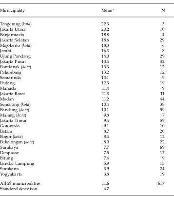
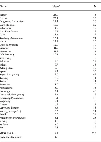
Tables 2a and 2b also indicate that urban firms (those located in municipalities) have slightly higher bribe rates than non-urban ones (located in districts).4
How-ever, there is a wide range of variation in average bribe rates across districts, from just 3.8% in Yogyakarta (table 2a) to 25.0% in Banjar (table 2b). One explanation
TABLE 1 Bribe Rates by Firm Typea (bribes as % of production costs)
Characteristics Mean N
Size (annual sales revenue)
Small (< Rp 1 billion) 10.4 488
Smaller-medium (Rp 1–5 billion) 11.6 322
Larger-medium (Rp 5–10 billion) 9.6 324
Large (> Rp 10 billion) 8.2 195
Sector
Manufacturing 9.3 646
Agribusiness 10.3 69
Services 11.3 618
Location
Urban (kota) 11.8 617
Non-urban (kabupaten) 10.3 716
Export orientation
Exporterb 9.7 371
Non-exporter 10.4 962
Ownership
Foreignc 12.0 167
Domestic 10.2 1,164
District oil/gas resources
Oild 12.8 162
Non-oil 9.8 1,171
aTotals in each group should be 1,333, which is the number of firms reporting bribes, but
there are some missing values. For example, there are 4 firms in the first group for which there is no information on size.
bExports at least 5% of sales.
cForeign ownership share at least 5% of total. dOil and gas output at least 5% of regional GDP.
Source: Calculated from the Special Survey on Governance, LPEM–FEUI.
for this is that some districts have a very small number of firms (less than 10) in the sample and, as a consequence, the average bribe is very sensitive to the pres-ence of outlier firms. Banjarmasin, for example, recorded a high bribe rate of 18.8%, but the sample size was only seven firms—of which just four reported positive bribes.
TABLE 2a Mean Bribe Rates across Municipalities (bribes as % of production cost)
Municipality Meana N
Tangerang (kota) 22.3 3
Jakarta Utara 20.2 10
Banjarmasin 18.8 4
Jakarta Selatan 18.6 29
Mojokerto (kota) 18.3 6
Jambi 16.3 8
Ujung Pandang 14.0 29
Jakarta Pusat 13.4 32
Pontianak (kota) 13.3 12
Palembang 13.2 12
Samarinda 13.1 9
Padang 12.3 19
Manado 11.4 9
Jakarta Barat 11.3 11
Medan 11.2 44
Semarang (kota) 10.4 38
Bandung (kota) 10.1 59
Malang (kota) 9.8 7
Jakarta Timur 9.4 59
Gorontalo 9.1 10
Batam 8.7 20
Bogor (kota) 8.4 12
Pekalongan (kota) 8.0 22
Surabaya 7.7 69
Denpasar 7.5 17
Bitung 7.4 9
Bandar Lampung 5.9 15
Surakarta 3.9 24
Yogyakarta 3.8 19
All 29 municipalities 11.6 617
Standard deviation 4.7
aThe mean is calculated only from firms reporting positive bribes. Unlike those in table 1,
the mean values shown here are unweighted: a district with 10 firms counts equally with another with 30.
Source: Calculated from the Special Survey on Governance, LPEM–FEUI.
Local Government Responses
The second part of the SSG involved in-depth interviews with top officials of dis-trict governments. Of the 64 governments surveyed, nearly half (including all the oil-rich districts) claimed that PAD receipts under the new decentralisation arrangements were not high enough to finance even routine expenditures—let alone development (capital) expenditures—while in another 14 they were consid-ered adequate to cover only the routine budget.5So the tendency to raise extra
revenue by introducing various new taxes (Lewis 2003) is not surprising. Some district governments are aware that the creation of too many taxes and levies will hurt the business sector, but argue that they are hard pressed to find sufficient revenue to cover their increased responsibilities for service delivery. At the same time, presumably at least some of their officials are well aware of the scope for increasing their personal incomes through bribes from businesses wish-ing to avoid the payment of taxes and levies: each new tax creates an additional opportunity to boost one’s income by agreeing not to enforce payment. The greater freedom from central control resulting from decentralisation has seriously weakened an important constraint on this type of government behaviour at local level. It is worth noting that local government officials were still overwhelmed by decentralisation euphoria, and that an obsession with PAD as an indicator of ‘suc-cess’ was still visible at the time of the survey: responses suggested that the first priority of 50 of the 64 local governments surveyed was to increase levies and cre-ate new taxes.6
Corruption and the Business Sector
By contrast, the main concern of the business community is the need to stream-line taxes, levies, licensing procedures and so on. Most firms say they are pre-pared to pay taxes, but it is the creation of new taxes and levies, many of them overlapping, that causes headaches. The complaint is directed not at specific taxes or levies but at their overall number.
One case of a new ‘nuisance’ tax may illustrate this point. Many district gov-ernments have chosen to create a new levy on the use of diesel generators. Pre-dictably, this measure encountered strong opposition from both service firms (particularly hotels) and manufacturing firms, especially in off-Java areas, which argued that the electricity supply was so unreliable that they had to rely on their own generators. Levying the use of generators would increase their costs and thus jeopardise their competitiveness.7In many districts these protests were to no
avail, however, so firms then tried to reduce the impact of the levy by bribing inspectors to falsify the number of generators they owned—no doubt precisely the result intended by at least some of the officials involved in the levy’s intro-duction. The result was therefore to generate some revenue for the government and some bribe income for certain officials, with the cost borne by the firms in question.
The procedures for renewing business licences and permits are also a source of irritation for the business sector, since they are cumbersome and are invariably exploited by corrupt officials. In the course of the survey we came across one case of a firm that failed to renew its ‘disturbance’ licence on time,8 and was then
forced to pay a bribe of Rp 3 million to renew it. Some district governments have tried to streamline the licensing process by bringing it under one roof, but
TABLE 2b Mean Bribe Rates across Districts (bribes as % of production cost)
District Meana N
Banjar 25.0 5
Cianjur 22.1 15
Tangerang (kabupaten) 17.1 16
Lombok Barat 15.5 22
Sukabumi 14.7 17
Riau Kepulauan 13.7 19
Kutai 13.6 7
Bandung (kabupaten) 13.4 71
Maros 12.7 15
Musi Banyuasin 12.0 10
Gianyar 11.8 10
Mojokerto 11.7 24
Deli Serdang 10.1 24
Karawang 10.0 2
Sidoarjo 9.8 29
Bekasi 9.7 33
Batang Hari 9.7 10
Jepara 9.4 55
Bogor (kabupaten) 9.0 49
Badung 8.7 11
Bantul 8.5 11
Pasuruan 8.0 20
Purwakarta 8.0 15
Lamongan 7.4 40
Pontianak (kabupaten) 7.4 8
Semarang (kabupaten) 7.4 17
Magelang 7.1 6
Klaten 6.9 27
Lampung Tengah 6.6 15
Malang (kabupaten) 6.3 14
Gresik 5.5 28
Pekalongan (kabupaten) 5.1 28
Serang 4.6 6
Asahan 4.5 15
Pati 2.8 22
All 35 districts 9.7 716
Standard deviation 4.7
aThe mean is calculated only from firms reporting positive bribes. Unlike those in table 1,
the mean values shown here are unweighted: a district with 10 firms counts equally with another with 30.
Source: Calculated from the Special Survey on Governance, LPEM–FEUI.
progress is very slow. Firms are still required to go to different offices to renew various permits, or at least to obtain ‘letters of recommendation’. One bus com-pany, for example, needed to acquire from different offices a ‘disturbance’ permit, a business registration permit and an advertising permit, as well as to register its land and buildings. Yet even after all this was done (presumably with attendant bribe payments), there was no guarantee that a new permit would not be needed for some other purpose. Sometimes officials from agencies that had already issued permits might even come back and ask for additional bribes.
A MODEL OF BRIBERY OF GOVERNMENT OFFICIALS
In order to guide the empirical work, we develop a simple model of bribery, as follows. Each firm faces costs imposed on it by governments—in particular, taxes and the costs of compliance with various regulations. We assume that govern-ment officials responsible for administering taxation and regulations have a level of discretion that enables them to grant ‘dispensations’ to firms, allowing them to pay less tax and to comply less than fully with the regulations. Such dispensa-tions can be bought by paying a bribe to the relevant officials, as in the case of the diesel generator tax just mentioned. Apart from the cost of bribe negotiations, the gain to the firm is the net dispensation: that is, the dispensation net of the bribe paid to obtain it.
Both the official and the firm gain from the transaction. What is at issue is how the aggregate gain is divided up, and this will be the focus of negotiation between the two sides. This process is analogous to bargaining in traditional markets over the price of fruit, for example. Both buyer and seller stand to gain from the trans-action, but the allocation of the aggregate gain between the two parties depends on the price they agree on. Each party is willing to devote some time to bargain-ing in order to get a better deal than that first offered by the other. The strategy of each party is to try to persuade the other that the transaction would be of only marginal benefit at the price offered, with the implication that if the price moves adversely then the benefits will disappear, and the transaction will not go ahead. Each party relies on his or her bargaining experience to distinguish bluff from reality in what the other party is saying, and thus to arrive at the best possible deal at the end of the process. And so it is with the official and the firm as they set about consummating a deal in which the firm benefits from a reduction in the costs imposed on it by the government, in return for a bribe paid to the official.
In trying to understand the determinants of the size of bribes paid (after scal-ing for the size of the firm as indicated by, for example, its total annual produc-tion costs), it makes sense to focus on the firm’s profitability.9When bribery is
systemic and ongoing, the upper limit to bribes that can be extracted from a firm is determined by its supernormal profit—that is, profit over and above the level required to keep it operational. Government officials could demand bribes in excess of supernormal profits, but from the firm’s point of view it would be preferable to go out of business than to pay up. This would be analogous to the food buyer and the market trader failing to agree on a mutually acceptable price for some fruit. Our fundamental hypothesis, then, is that the more profitable the firm, the higher the bribes it will pay (again after scaling profits and bribes for the size of the firm).
A second consideration is the amount of time that managers of the firm spend in negotiations with government officials. We assume that such negotiations are primarily concerned with the price they have to pay to obtain dispensations, as described above. Firms operating in competitive industries are much alike. They operate in similar fashion and earn normal profits, and we would expect there to be some standard level of bribes that they all pay to officials; these standard bribes would then be incorporated into the firm’s normal cost structure. Officials would realise that there is no point in demanding larger bribes from such firms: this will only result in an unnecessarily long bargaining process (at the end of which the bribe ends up being the industry standard) or in the closure of the firm.
On the other hand, firms that have some market power (having differentiated themselves from others by introducing a new product or employing superior technology, for example) are likely to be earning supernormal profits, but the very fact that they are different from other firms means that it will be hard for government officials to guess how high their profits are, and how their profitabil-ity evolves over time. Given this lack of key information, our second hypothesis is that officials will start out demanding relatively high bribes for any given dis-pensation they may offer. At the same time, the firms themselves will request larger dispensations or offer lower bribes, hoping that they will be able to con-vince predatory officials that they are not as profitable as they appear. The result will be a longer process of negotiation than usual to settle on the net dispensa-tion. Thus we expect that high profitability will be associated with a need for greater management effort in negotiations with officials, resulting, in turn, in bribe rates being positively correlated with management time spent in negotia-tions.
A third feature of the bribery model is the possibility that the bureaucracy will introduce more regulations and taxes in industries in which they suspect that firms typically earn above normal profits. Each new tax or regulation introduced provides a new instrument for predation by corrupt officials—for example, by withholding (or delaying the issue of) permits necessary to operate a business, or by forcing the firm to incur additional costs in the name of public safety or envi-ronmental protection. On the other hand, once the official is armed with one instrument that effectively confers the power to close down a firm, the introduc-tion of another similar instrument offers no addiintroduc-tional power to extract bribes from it. In reality, therefore, if there are multiple regulations it is very likely that they have been introduced by multiple arms of the bureaucracy. The maximum that can be extracted from a firm, however—if it is not to be driven to close—is limited by its supernormal profit, no matter how many predators there are. It is possible, therefore, that the introduction of new regulations will leave the aggre-gate bribe payment roughly unchanged, and merely spread it more thinly among a larger number of officials.
A fourth aspect is closely related to the third. There may be a concern that, even if a bribe is paid, the official will not be able to deliver on the promised dispensa-tion. Since the expected value of the dispensation will be less than the promised value in these circumstances, the bribe the firm is prepared to pay will also be less.10On the other hand, whether the firm actually receives what is promised by
one official probably has less to do with that official’s actions than with
tion for bribes by others from different parts of the bureaucracy, as in the case of the bus company mentioned above. Thus, if there is a lack of confidence on the part of the firm that it will receive the promised dispensation, it will pay a rela-tively small bribe—but in circumstances in which it expects to have to pay bribes to a number of other officials as well. Thus there may be no clear correlation between the overallbribe rate and the perceived probability of bribes being effec-tive.
Various characteristics of the firm itself might be expected also to be related to its payment of bribes. Firms that are successful in negotiating relatively low bribes because of their bargaining skill will be more profitable than others that are identical in other respects, and so may be expected to live longer and to grow faster (given that growth depends heavily on reinvested profit). In other words, the bribe rate is likely to be negatively correlated with the age and size of the firm, other things being equal. A closely related possibility is that officials who take a long-term view of their income from bribery will realise that it is in their own interests not to impose excessive costs on firms over which they exercise regula-tory authority: if such firms go out of business, or relocate, the income source will be lost and effort will need to be expended to replace it. Relationships developed over lengthy periods between older firms and corrupt officials may therefore be characterised by lower bribe rates.
Interregional differences in resource endowments may influence corrupt behaviour. The impact on the quality of governance by local officials of the new decentralisation arrangements that redirect a large share of natural resource rev-enues back to the source districts remains to be seen, but it may not differ greatly from the impact of a resource boom on government officials in other countries. There is a large body of literature suggesting that corruption tends to be more entrenched in resource-rich regions (Gelb and associates 1988; Karl 1999; Auty 2001; Eifert et al. 2002). In particular, Karl (1999) suggests that a large and concen-trated rent source in national income could transform a country into a ‘rentier state’, and that the sudden emergence of large revenue streams could be used to underpin kleptocratic governments.
In the present context, some of the rents from natural resources are likely to spill over and be captured by firms within the districts concerned—particularly those that deal directly with firms involved in natural resource exploitation. In such cases, supernormal profits will result from firms’ closeness to officials in the industry in question, rather than from their more purely entrepreneurial capabil-ity, and so these officials are likely to have a more accurate knowledge of the size of the profits available for expropriation. This strengthens their hand in the bar-gaining process, and can be expected to generate higher bribe rates in these dis-tricts.
The sector and location in which the firm operates may affect the bribe rate. A representative of the Indonesian Hotels and Restaurants Association (Persatuan Hotel dan Restoran Indonesia, or PHRI) suggested that businesses of this kind obtain most of their revenue in cash on a daily basis, making them easier targets for petty extortion by officials than manufacturing and agribusiness firms that receive payments for sales less frequently, and often not in the form of cash. It is also possible that industry associations might exert some influence to protect their members from predatory officials, and that the effectiveness of such
ations differs between sectors. The data presented in tables 2a and 2b also suggest rather lower bribe rates in non-urban areas. We can see no obvious reason why bribe rates should differ by location, however, and the observed differences in these tables may simply be masking the effect of differences in size or sector rep-resentation in urban and non-urban areas.
There may be differences in the extent of bribes paid depending on whether the firm produces for the export market or whether it is foreign owned. It is dif-ficult to speculate on the relationship between export orientation and the pay-ment of bribes, but one possibility is that if firms locate in export-processing zones where there are fewer formal requirements for permits of all kinds, they may be protected from the necessity of paying bribes. On the other hand, it was argued above that it is not necessary to have numerous regulations in order to maximise the total bribes paid by firms, so even if firms in export-processing zones face fewer regulatory obstacles there may be little difference in the total amount of bribes they pay.
Foreign firms may be less likely to pay bribes if their corporate culture is averse to corrupt dealings with officials, or because of restrictions imposed by their head-quarters. For example, the US and some countries in the European Union have laws that explicitly forbid firms to bribe foreign government officials.11In
addi-tion, even though foreign ownership may make a firm more vulnerable to extor-tion by the bureaucracy, foreign firms typically have domestic partners chosen precisely for their ability to ward off bureaucratic predation. Thus the burden of vulnerability may take the form of a stream of dividends to domestic partners that contribute no capital to the firm, rather than bribes paid direct to corrupt officials. These considerations suggest a negative relationship between bribes paid and for-eign ownership.
EMPIRICAL INVESTIGATION
In this section we employ the SSG data set to examine the extent of corruption at district level in 2001–02, immediately after the laws on decentralisation went into effect. Unfortunately, we do not have data on the corrupt behaviour of local bureaucrats under the previous regime, which could be used to measure firms’ responses to changes in bureaucrats’ behaviour consequent on decentralisation. Instead we attempt to obtain a snapshot of the post-decentralisation determi-nants of bribery, controlling for firm, location and industry characteristics.
To ascertain the determinants of bribes paid by firms, a bribe function based on the model described above is estimated econometrically. The estimating equation is:
(1)
where B is the level of bribery; X is a vector of ‘government variables’ that describe the relationship between firms and government officials; Yis a vector of ‘firm variables’; Zis a vector of ‘district variables’; uis the error term; and a, b, c
and dare parameters to be estimated.
The dependent variable is the bribe rate, defined as bribe payments as a per-centage of production costs. The definitions of the government-related,
firm-B=a+b.X+c.Y+d.Z+u
related and district-related variables hypothesised to determine the bribe rate are set out below (for precise details see appendix 1).
Government-related Variables
The first four explanatory variables—tax payments, time spent, regulatory burden
and bribe efficacy—reflect government-related aspects of the environment faced by firms (see appendix 1 for details of the survey questions).
Tax Payments. The model predicts that bribes will be larger for firms with higher profitability. In the absence of data on the latter, we use as a proxy infor-mation on a firm’s tax payments(as a proportion of annual production costs).12
Time Spent. The time spentvariable captures the proportion of their time firms’ managers spend negotiating with officials to obtain the most advantageous net dispensations. Respondents were asked to state, on a scale of one to six, the pro-portion of productive time devoted by management to interactions with officials in order to ‘smooth business operations’ in relation to regulatory matters (includ-ing taxation).
Regulatory Burden. The model suggests that each different arm of the bureau-cracy may introduce regulations (and taxes) as instruments for generating bribe income for their officials. The regulatory burdenis proxied here by the number of operational licences required for normal business operations.
Bribe Efficacy. Respondents were asked to assess the likelihood that payment of bribes would guarantee receipt of ‘promised services’ (i.e. dispensations, in the terminology we have employed here), on a six-point scale of responses ranging from ‘never’ to ‘very often’.
Firm-related Variables
The next set of explanatory variables reflects characteristics of the firms them-selves.
Age. Ageis calculated from the date the firm was founded.
Size. Sizeis indicated here by firms’ annual sales in the previous year. Three dummy variables are created to represent smaller-medium, larger-medium and large categories, while the small category is used as the reference case.13
Location. A location dummy variable is included to distinguish firms in urban areas (kota) from those in non-urban areas (kabupaten).
Sector. Industry sector dummy variables are included to distinguish manufac-turing and services firms, while agribusiness is the reference case.
Export Orientation. Export orientation is represented by a dummy variable, having the value 1 for exporters and 0 otherwise. A firm is classified as an exporter if it exports at least 5% of its output.
Foreign Ownership. Foreign ownership is represented by a dummy variable, having the value 1 for foreign firms and 0 otherwise. A firm is classified as for-eign owned if it has at least 5% of its shares in forfor-eign hands.
District-related Variable
Oil-Rich Districts. We investigate the link between bribery and natural resource endowment by focusing on Indonesia’s most valuable such resources, oil and gas.14‘Oil-rich districts’ are those for which the value of oil and gas production
exceeded 5% of regional GDP in 1999; the oil dummy takes the value 1 for these
districts and 0 for others. (According to this definition there are five oil-rich dis-tricts among the 64 surveyed: Kutai, Riau Kepulauan, Musi Banyuasin, Batang Hari and Jambi.)
Consistency Checking of Reported Government-related Variable Data
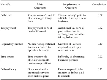
For the purpose of consistency checking, we performed a correlation analysis between responses to the main question for each core variable and responses to the supplementary question for that variable. In particular, we looked for per-verse correlations within hypothesised relationships as a sign of inconsistency.15 The hypothesised relationships could also come from logical associations between two variables.16Considering the sensitivity of the bribery issue, which might have induced the respondents to hide the true answer, we used a thresh-old of around 0.2 (in absolute value) to judge whether two variables had a sensi-ble correlation.
Table 3 shows that all correlation coefficients are well within the range of our criterion for a reasonable degree of association. Also, since no perverse relation-ship is observed, at least in the key variables, the survey responses can be consid-ered to be reasonably consistent. The highest correlation (0.67) is between ‘grease money’ to get things done and ‘grease money’ to set up a new business. At the lowest end (0.22) are two coefficients measuring, respectively, the correlation between time spent with bureaucrats and the difficulty of obtaining a new
busi-Bribe rate officials to set up a new business
TABLE 3 Consistency Checking for the Key Variablesa
Variable Main Supplemenary Correlation
Questions Questions
aSee appendix 1 for precise questions.
ness permit, and the correlation between two measures of the uncertainty associ-ated with paying bribes. These coefficients are reasonable, however, given the fact that this is a firm-level cross-section study. The correlation coefficient between time spent and the difficulty of obtaining a business permit is not as high as expected, but time spent itself presumably encompasses a broader range of activ-ities than merely applying for new business permits. The correlation between tax payments and willingness to pay additional tax in exchange for no-bribe behav-iour is quite high (0.52). Finally, the number of operational licences required for normal operations has a fairly high correlation (0.40) with the level of bribes needed to set up a new business.
ECONOMETRIC APPROACH AND RESULTS
As noted earlier, of 1,808 respondents, only 1,333 acknowledged that they paid bribes, while the rest claimed not to do so. This presents a problem for econo-metric analysis. Application of the ordinary least squares (OLS) method would require observations of firms reporting zero bribes to be discarded, which would result in the loss of important information, and might bias the estimated bribe function. One possible way to remedy this problem is to use the Tobit estimation procedure (Greene 1993: 694). This procedure is used when a substantial number of observations of the dependent variable are zero or are clustered closely around zero. However, the use of this procedure may also produce biased estimates if the zero observations of the dependent variable are actually substituting for un-observed positive values. In the present context, some firms may incorrectly have reported zero bribes because they were too embarrassed to admit involvement in corrupt behaviour.17Thus the Tobit procedure may not reveal the true functional
relationships that constitute the bribe equation.
The problem could be handled easily if we knew that all firms reporting zero bribes were not telling the truth. In this case we could look for a pattern of rela-tionships between non-disclosure of bribes and the posited determinants of bribery already outlined, by applying a Heckman-type selection or truncation model, in which the decision about whether to reveal the payment of bribes is taken into account when estimating the model (Heckman 1979). In essence, the Heckman procedure uses the Probit method to retrieve the predicted (positive) value of a false zero, and then uses this predicted value as an additional inde-pendent variable in the OLS regression, as a correction factor. Unfortunately, however, ours is not a simple case of truncation, because the zero bribe responses may be a mixture of those who did not pay any bribes and those who did so but chose not to admit it, so this approach may also fail to reveal the true functional relationship.
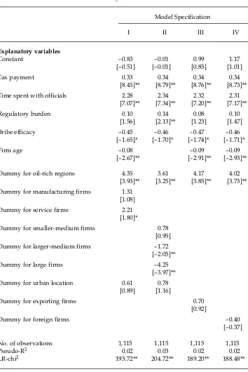
A full econometric treatment to resolve this problem is beyond the scope of the present paper. Our approach is to undertake a kind of sensitivity analysis, by run-ning all three kinds of regressions and comparing the results—thus allowing us to attempt to infer the direction of bias. The coefficient of time spent in equation (1) appears to play a central role in assessing bias, since it is the most sensitive to change in the estimation procedure. The Tobit, Heckman and OLS estimates for a number of specifications of the bribe function are shown in tables 4, 5 and 6, respectively.
Although 1,808 firms were interviewed, for nearly one-third of these there was insufficient information to allow their inclusion in the sample, leaving a total of 1,115 usable observations; of these, 1,027 reported positive bribe rates. Table 4 presents the Tobit estimates for the larger group, based on the assumption that the zero bribe observations are correct. Table 5 presents the results of the two-stage Heckman procedure, assuming that the zero observations are false.18 As
explained above, the first stage involves a Probit regression that shows the influ-ence of each of the independent variables on the firm’s decision about whether to reveal having paid bribes. The dependent variable takes the value of 1 if the reported bribe payment is positive, and 0 otherwise. For each model specifica-tion, the first-stage result is accompanied by its corresponding second-stage OLS regression in the second column. The second stage uses the information obtained in the first stage to undertake a modified OLS regression. The lambda is calcu-lated from the Probit equation, and is used as an additional independent variable in the OLS regression to account for the assumed false zero bribe observations.19
Table 6 presents the OLS regressions for the smaller group that excludes firms reporting zero bribe payments.
These three econometric approaches yield generally consistent results in respect of most of variables, for which the coefficients are similar, as is the pattern of statistical significance. The main exception, so far as statistically significant coefficients are concerned, is the time spentvariable: the coefficient obtained using OLS (about 1.8–1.9) lies between those obtained using the other two procedures (about 2.3 for Tobit and 1.5–1.6 for Heckman). The Tobit procedure produces a higher coefficient because the regression function attempts to accommodate many observations that cluster at a zero bribe rate. On the other hand, the coeffi-cient derived from the Heckman procedure is relatively small because of the assumption that some of the zero bribe rates reported are actually false, and are corrected to positive values. The other exception is the coefficient on large firm size, which is 4.3 in the Tobit estimates, but about 4.0 in the OLS and 3.8 in the Heckman estimates.
Given the likelihood that the zero bribe rate observations include both true zeros and actual positive values, it is probable that the Heckman procedure pro-duces less bias than either OLS or Tobit. Judging from the direction of bias in the
time spent coefficient, the Tobit procedure appears to be the least reliable. The coefficient on the variable lambda in the Heckman model is insignificantly differ-ent from zero, however, which implies that the modified OLS regression obtained from this procedure is not statistically different from the unmodified OLS regres-sion reported in table 6, probably because many of the zero bribe observations are actually correct.
The first-stage Probit equation concerning the decision about whether to reveal the payment of bribes does provide valuable information, nevertheless. Note, for example, that firms that perceive a high degree of bribe efficacy are significantly less likely to reveal the payment of bribes, suggesting that many of the zero bribe observations are indeed false.20The equation also suggests that older firms are
significantly less likely to reveal paying bribes. Those firms are survivors in part because of their ability to negotiate more generous net dispensations with offi-cials, but they also appear to be reluctant to reveal their ongoing relationships with corrupt officials. The other interesting result from the first-stage Heckman
TABLE 4 Determinants of Bribe Rates: Tobit Estimatesa
Model Specification
I II III IV
Explanatory variables
Constant –0.83 –0.01 0.99 1.17
[–0.51] [–0.01] [0.85] [1.01]
Tax payment 0.33 0.34 0.34 0.34
[8.45]** [8.79]** [8.76]** [8.73]**
Time spent with officials 2.28 2.34 2.32 2.31
[7.07]** [7.34]** [7.20]** [7.17]**
Regulatory burden 0.10 0.14 0.08 0.10
[1.56] [2.13]** [1.23] [1.47]
Bribe efficacy –0.45 –0.46 –0.47 –0.46
[–1.65]* [–1.70]* [–1.74]* [–1.71]*
Firm age –0.08 –0.09 –0.09
[–2.67]** [–2.91]** [–2.93]**
Dummy for oil-rich regions 4.35 3.61 4.17 4.02
[3.93]** [3.25]** [3.85]** [3.73]** Dummy for manufacturing firms 1.31
[1.08]
Dummy for service firms 2.21
[1.80]*
Dummy for smaller-medium firms 0.78
[0.95]
Dummy for larger-medium firms –1.72
[–2.05]**
Dummy for large firms –4.25
[–3.97]**
Dummy for urban location 0.61 0.78
[0.89] [1.16]
Dummy for exporting firms 0.70
[0.92]
Dummy for foreign firms –0.40
[–0.37]
No. of observations 1,115 1,115 1,115 1,115
Pseudo-R2 0.02 0.03 0.02 0.02
LR-chi2 193.72** 204.72** 189.20** 188.48**
aEstimates are for all usable observations (1,115), and are based on the assumption that the
zero bribe observations are correct. Figures in parentheses are t-ratios. **significant at 5%; * significant at 10%.
TABLE 5 Determinants of Bribe Rates: Heckman Estimatesa
Regression Specification I Specification II
Equation
Probit OLS Probit OLS
Dependent variable Reveal bribe Bribe Reveal bribe Bribe
or not rate or not rate
Explanatory variables
Constant 1.43 0.45 1.17 1.94
[4.62]** [0.20] [5.61] [0.76]
Tax payment –0.003 0.38 –0.003 0.39
[–0.54] [9.36]** [–0.36] [9.72]**
Time spent with officials 0.28 1.46 0.28 1.59
[4.23]** [2.10] [4.33]** [2.25]**
Regulatory burden –0.005 0.12 –0.004 0.16
[–0.42] [1.85]* [–0.36] [2.40]**
Bribe efficacy –0.15 0.10 –0.14 0.05
[–3.30]** [0.22] [–3.29] [0.11]
Firm age –0.01 –0.05
[–2.10]** [–1.04]
Dummy for oil-rich regions 0.37 3.07 0.32 2.63
[1.68] [2.20] [1.41] [2.01]**
Dummy for manufacturing firms –0.13 1.76 [–0.55] [1.42]
Dummy for service firms –0.06 2.56
[–0.25] [2.07]**
Dummy for smaller-medium firms 0.12 0.34
[0.76] [0.39]
Dummy for larger-medium firms –0.08 –1.56
[–0.51] [–1.85]*
Dummy for large firms –0.23 –3.75
[–1.19] [–3.15]**
Dummy for urban location 0.07 –0.08 0.21 0.14
[0.92] [–0.10] [1.71]* [0.17]
Lambda –5.99 –4.61
[–0.55] [–0.42]
Wald-chi2 196.09** 201.88**
No. of observations 1,115 1,115
Censored observations 88 88
Uncensored observations 1,027 1,027
aEstimates are for all usable observations (1,115), and are based on the assumption that the
zero observations are false. Figures in parentheses are t-ratios. **significant at 5%; * significant at 10%.
equation (specification II) is that urban firms are more likely to reveal paying bribes than non-urban—although the coefficient is only significant at the 10% level.
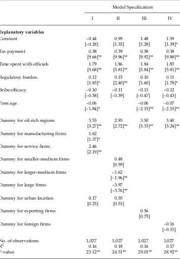
Since the Heckman procedure does not improve on the simple OLS results, sta-tistically speaking, the remainder of the discussion is based on the results of the four unmodified OLS regressions (table 6). The coefficient of the tax payments
variable is positive, as expected, and significant at the 5% level for all four speci-fications of the model reported here. It may seem ironic that higher tax payments go hand in hand with larger bribes, given that the purpose of paying bribes is (in part) to reduce a firm’s tax assessment. The model suggests the explanation for this result is that firms that pay large amounts of tax relative to their size are those with relatively high (supernormal) profits, which makes them an attractive target for predatory officials.
The coefficient for time spentis also positive and significant at the 5% level in all model specifications. This is consistent with the model’s prediction, based on the reasoning that there is likely to be greater uncertainty on the part of officials as to the precise level of profits of firms that stand out as more profitable than, but different from, other firms, thus making it worthwhile for both parties to invest more time in the bargaining process.21
The coefficient for regulatory burden is positive, as suggested by the model, based on the idea that the regulatory environment is to some extent tailored to bureaucratic perceptions of profitability in the relevant industry. Statistically speaking, this is a weaker explanatory than the time variable, however, although in specifications I, II and IV the coefficient is still significant, at least at the 10% level.22This lends weight to the argument that proliferation of taxes and
regula-tions results in bribe income being spread over officials from several arms of the bureaucracy, with little or no increase in total bribe payments by firms—whose capacity to make such payments is limited by their profitability.
The bribe efficacyvariable coefficient is not significantly different from zero in any model specification except the presumed less reliable Tobit results (table 4). The sign of the coefficient, however, is in line with the rather weak prediction of the model that lack of confidence in the ability of officials to deliver promised dis-pensations will be inversely related to bribe levels.23Our preferred explanation
for the lack of a strong relationship is that low bribe efficacywill result in low bribe rates for the official in question, but will also reflect the fact that many officials with veto power will need to be bribed—such that the total bribe payment will be little different from what it would have been if a single official had this veto power.
The coefficient for age of the firm is negative and significant at the 5% or 10% level for the three model specifications in which this variable is included, con-firming the hypothesis that older firms pay somewhat lower bribes. The coeffi-cients of the firm size dummy variables are also consistent with the model’s predictions.24 For smaller-medium firms the coefficient is insignificant in all
model specifications, but the coefficients for larger-medium and large firms are negative and significant at the 5% level, suggesting that bribe rates decline with increasing firm size.
The oildummy has positive coefficients, significant at the 5% level in all model specifications, suggesting strongly that bribe rates are indeed higher in oil-rich
TABLE 6 Determinants of Bribe Rates: OLS Estimatesa
Model Specification
I II III IV
Explanatory variables
Constant –0.44 0.99 1.48 1.59
[–0.28] [1.35] [1.28] [1.39]*
Tax payment 0.38 0.39 0.38 0.38
[9.66]** [9.96]** [9.92]** [9.88]**
Time spent with officials 1.79 1.86 1.84 1.83
[5.68]** [5.81]** [5.84]** [5.81]**
Regulatory burden 0.12 0.15 0.10 0.11
[1.83]* [2.40]** [1.60] [1.78]*
Bribe efficacy –0.10 –0.11 –0.13 –0.12
[–0.38] [–0.39] [–0.47] [–0.43]
Firm age –0.06 –0.06 –0.07
[–1.84]* [–2.15]** [–2.15]**
Dummy for oil-rich regions 3.53 2.93 3.50 3.40
[3.27]** [2.72]** [3.33]** [3.24]** Dummy for manufacturing firms 1.62
[1.37]*
Dummy for service firms 2.46
[2.19]**
Dummy for smaller-medium firms 0.48
[0.59]
Dummy for larger-medium firms –1.62
[–1.96]**
Dummy for large firms –3.97
[–3.76]**
Dummy for urban location 0.17 0.35
[0.25] [0.53]
Dummy for exporting firms 0.56
[0.75]
Dummy for foreign firms –0.16
[–0.15]
No. of observations 1,027 1,027 1,027 1,027
R2 0.16 0.18 0.16 0.17
F-value 23.12** 24.51** 29.01** 28.92**
aEstimates are for the smaller group (1,027) that excludes firms reporting zero bribe
pay-ments. Figures in parentheses are t-ratios. **significant at 5%; * significant at 10%.
districts. Although the firm interviews tended to suggest that corrupt behaviour of officials in oil-rich districts is on the increase, we have no hard evidence of this. What we can say now, with some confidence, is simply that officials in oil-rich districts appear to be more corrupt than those in non-oil districts.
The coefficients of the industrysectordummies suggest that firms in the serv-ice sector do indeed pay more in bribes than those in manufacturing and agribusiness. This result conforms with the data in table 1. A possible explanation for this result, however, is that it is a statistical artifact. There may be correlation between the sector and size dummies: manufacturing and agribusiness firms tend to be larger, and thus have lower bribe rates than those in the service sector.
The coefficient of the urbanlocationdummy is positive, but insignificant at the 10% level. In other words, the data suggest that location has no impact on the bribe rate once other factors are taken into account.
We had hypothesised that export-oriented firms may enjoy some protection from bureaucratic extortion by locating inside industrial or export-processing zones. The coefficient of the dummy variable for exporting firms actually turns out to be positive, however, although it is not significantly different from zero. A better test of this hypothesis would need to distinguish firms located in such zones; many exporters in our sample were located outside them.
Finally, the coefficient of the dummy variable for foreign ownership is also insignificant, suggesting that there is no difference in bribe rates between foreign firms and their domestic counterparts once other factors are taken into account. This is consistent with the possibility that extortion of such firms is effectively by way of their domestic partners, rather than directly.
Relative Importance of the Determinants of Bribe Rates
The upper part of table 7 shows the contribution to the bribe rate of each of the independent non-dummy variables, evaluated at their respective mean values, for our two preferred specifications of the OLS model; the export orientation and foreign ownership variables (with coefficients insignificantly different from zero) are absent from these specifications. The reference cases are those of firms in a non-oil, non-urban area; for model I this firm is in the agribusiness sector, and for model II it is a small firm. The estimated bribe rates for these reference firm cate-gories are 7.9% and 10.7%, respectively.
If we focus on differences across sectors(model I), we find that the bribe rate increases to 8.7% for manufacturing firms and then to 9.1% for those in the serv-ices sector. Alternatively, if we allow firms’ sizeto vary (model II), we observe that the bribe rate falls to 10.3% for both larger-medium firms and larger firms. The bribe rates for the reference firms increase to 8.3% and 11.1% (for models I and II, respectively) if they are located in oil-rich districts. Urban location generates slight increases in bribe rates; recall, however, that the positive coefficients on this variable were insignificantly different from zero.
In both specifications, the contribution of the tax payment variable is the largest, accounting for about 5 percentage points—or roughly 60% and 47% of the total bribe rate in models I and II respectively. The time spentvariable also provides large contributions to the bribe rate in both specifications. In model I, for example, the absolute contribution of time spent to the predicted value of 7.9% for the reference firm bribe rate is 4 percentage points, or about 51% of the
total (38% in model II). By contrast, the other variables make only minor contri-butions to the bribe rate.
CONCLUSIONS AND POLICY IMPLICATIONS
We have tried in this paper to shed some light on the nature of corrupt relation-ships between firms and government officials at the district level in the more decentralised system of government created by the enactment of the laws on regional autonomy. We developed a simple model in which firms seek to reduce
TABLE 7 Contributions of Each Variable to Overall Bribe Rates: OLS Estimatesa
Mean Value Coefficient Contribution to
N = 1,027b Bribe Rate
(%)
Model Specification I II I II
Explanatory variables
Constant 1 –0.44 0.99 –0.4 1.0
Tax payment 12.49 0.38 0.39 4.7 5.0
Time spent with officials 2.23 1.79 1.86 4.0 4.1
Regulatory burden 5.80 0.12 0.15 0.7 0.9
Bribe efficacy 2.47 –0.10 –0.11 –0.2 –0.3
Firm age 13.51 –0.06 –0.8
Bribe rates for reference firms Agribusiness firms in non-urban,
non oil-rich districts 7.9
Small firms in non-urban,
non-oil-rich districts 10.7
Reference firm bribe rates adjusted for firm size
Smaller-medium 10.9
Larger-medium 10.3
Larger 10.3
Reference firm bribe rates adjusted for firm sector
Manufacturing 8.7
Services 9.1
Reference firm bribe rates adjusted for oil-rich districts 8.3 11.1
Reference firm bribe rates adjusted for urban locations 8.0 10.9
aThe constant term, bribe efficacy variable and dummy variables for smaller-medium
firms, manufacturing firms and urban locations are not significant.
bMean values are calculated only for the OLS sample (N = 1,027). The OLS sample is
smaller than the full sample of those reporting positive bribes (N = 1,333) because of miss-ing values of independent variables.
the costs imposed on them in the form of taxes and regulations, by offering bribes to government officials. The latter have some discretion to grant ‘dispensations’ in return for bribe payments, the effect of which is to reduce such costs.
In determining what bribe they will accept for a dispensation of a given value, officials are guided by their estimates of a firm’s profitability. They demand high bribes from firms with high profits, but will accept low bribes from firms with low profits: to do otherwise would be to drive the latter out of business. But since true profitability can only be guessed at by officials, and since firms have a strong incentive to understate their profits in order to escape with a lower bribe for a given dispensation, both sides need to spend time in negotiation until agreement is reached. We argue that higher profits tend to be earned by firms that differenti-ate themselves from others, and that this aspect makes it more difficult for officials to judge their profitability. In such circumstances there is more to be gained from a longer period of bargaining than would be the case with a more ‘normal’ firm, which could be expected to earn a normal profit and to pay a more standard bribe.
The main predictions of the model are that both bribes and the time spent in negotiations over bribes will be positively related to firms’ profitability. The implication is that we expect a positive relationship between bribes, on the one hand, and both tax payments as a percentage of annual production costs (which we take as a proxy for profitability) and time spent in negotiations with officials, on the other. These predictions were borne out by the empirical analysis. The neg-ative and significant relationships between bribes paid and the age and size of firms are also consistent with the argument that firms’ profits are the key deter-minant of the bribes they pay: firms that are successful in negotiating more favourable bribe/dispensation packages with the bureaucracy will be more prof-itable, and therefore will live longer and grow larger.
The business sector complains that decentralisation has prompted local gov-ernments to create many new regulations and nuisance taxes. These, it argues, have been accompanied by an increase in corrupt behaviour in the form of demands for bribes or indefinite regulatory delays that effectively convey the message that bribes will be needed if such delays and their associated costs are to be avoided. The hypothesis that the bureaucracy boosts the bribe incomes of its officials by customising taxes and regulations to perceived levels of industry profitability gained some support from the positive (albeit statistically weaker and quantitatively less important) relationship between the regulatory burden faced by firms and the size of their bribe payments. On the other hand, prolifer-ation of nuisance taxes and regulprolifer-ations appears to reflect competition between different arms of the bureaucracy for the limited total amount of bribes firms are capable of paying. This results in reduced efficacy of bribe payments: individual officials are unable to deliver promised dispensations because other parts of the bureaucracy have overlapping power to interrupt firms’ operations. This regula-tory fragmentation tends to spread bribe payments around, rather than to increase their aggregate amount, however. In short, the evidence is consistent with the possibility that firms have responded to the introduction of new taxes and regulations by paying smaller bribes to a greater number of individual offi-cials, such that total bribe outlays have not increased by much.
The notion that firms make no distinction between tax payments and the costs incurred in complying with regulations of all kinds suggests that governments
could collect more tax revenue if they reduced other cost burdens on firms by reducing the number of taxes, cutting back on unnecessary regulatory interven-tions, and acting more vigorously to restrain corrupt behaviour on the part of the bureaucracy. In turn, additional tax revenue could be used to raise civil servants’ salaries by more than these individuals’ loss of income from corrupt activity: this follows from the fact that a firm that is permitted to evade, say, Rp 1 million in tax will pay significantly less than Rp 1 million to the official offering the dispen-sation.
The observations above about bureaucratic competition for bribe payments suggest that this argument may be too optimistic, however. Tax offices located in the districts and municipalities are not part of local government but, rather, part of the central government machinery for collecting central government taxes such as corporate and individual income tax. Thus an important implication of the empirical analysis is that even if a district government succeeds in reducing corruption among its own officials (in the hope of attracting more businesses and generating more tax revenue at local level), central government tax officials may demand even larger bribes once it becomes clear that local officials are now extracting a smaller share of firms’ supernormal profits. An important consider-ation here is that officials from the centre may have little concern for the longer-term impact of corruption on the development of the district. Like other central government employees, they are subject to rotation to other districts, so it is not in their interests during their term of duty to make their present district of resi-dence more competitive in the long term by reducing the overall financial burden on firms from illegal imposts.
Finally, in line with the large body of literature on the behaviour of govern-ments in oil-producing countries, our study suggests that officials in oil-rich dis-tricts are somewhat more corrupt than those in non-oil disdis-tricts. This suggests that there is scope for significant gains through requiring larger royalty payments for the right to exploit natural resources, and through minimising the role of state-owned firms in this sector, since these provide an easy means of diverting natural resource wealth from its rightful owners—the general public. Our analy-sis does not enable us to conclude that oil-related corruption is a consequence of the new natural resource revenue sharing arrangements, despite some anecdotal evidence suggesting that corruption in oil-rich districts is on the increase. It will be interesting to observe whether these districts can use their expanded revenues to accelerate growth and bring about improvements in social welfare, despite the apparently higher level of official corruption.
NOTES
* I am grateful to Andrew MacIntyre and two anonymous referees, and to seminar par-ticipants at the Australian National University, for many helpful comments. All remaining errors are mine. I would like to thank the team members of the University of Indonesia’s Special Survey on Governance, in particular, Thia Jasmina, Ari Damayanti, Isfandiari Jafar, Isfandiarni, Suryadi and Eugenia Mardanugraha.
1 By mid 2004 the number of districts was closer to 400.
2 Firms that did not report paying bribes may in fact have paid them, of course, and this has important implications for the analysis. These are discussed in detail later.
3 These six districts, chosen to reflect the geographic spread of firms in Indonesia, were Bandung, Semarang, Malang, Palembang, Pontianak and Makasar.
4 The mean values shown here differ from those in table 1 in being unweighted: a dis-trict with 10 firms counts equally with another with 30.
5 Interestingly, the five municipalities of Jakarta are among very few that claim that PAD revenue is high enough to cover both routine and development expenditures. Motor vehicle tax is the most significant contributor to PAD.
6 Street lighting and hotels and restaurants were favourite targets. The street lighting tax is collected by the state electricity company (PLN) on behalf of the local government as a surcharge on its customers.
7 Any other tax levied on these firms would have the same impact, of course.
8 In effect, firms have to obtain permission to make a ‘disturbance’, such as noise, traffic congestion and waste discharge, before the business can be operated.
9 A well-known joke has it that, when asked why he robbed banks, a thief replied: ‘because that’s where the money is’. By analogy, the predator official can be expected to focus his attention on the firms he or she believes to be most profitable.
10 By analogy, if a rational buyer in a food market thinks that the seller’s weighing scales have a downward bias, she or he will offer a correspondingly lower price per kilogram of fruit.
11 The United States Foreign Corrupt Practice Act (1997); the OECD Convention on Com-bating Bribery of Foreign Public Officials in International Business Transactions (1999). 12 Tax offices in the districts and municipalities are not part of local government, but
rather of the central government machinery for collecting central taxes such as corpo-rate income tax. This has important implications for anti-corruption efforts at the dis-trict level, as we shall see later.
13 At the beginning of the survey, respondents were asked the value of annual sales, but the response rate was very low. It was therefore decided subsequently to ask respon-dents only to place their firms within one of these four size categories.
14 We performed several experiments in which the share of districts’ output of other nat-ural resource products in GDP—specifically, timber and minerals—was included in the regression, but these variables had very low statistical significance and so were dropped from the analysis.
15 For example, the variable used to measure bribe efficacy in the empirical model should correlate positively with alternative measures of bribe uncertainty, such as the firm’s ability to predict the bribe level.
16 For example, time spent with officials to smooth business operations should correlate positively with the degree of difficulty in getting officials to process business permit applications.
17 Recognising the secretive nature of bribery, we experimented with different question sequencing in the pre-test questionnaire. On the basis of these experiments, the ques-tion on bribes paid (as a percentage of producques-tion costs) was asked roughly half-way through the interview.
18 For the Heckman procedure, only the two best performing specifications (models I and II) are presented for comparison with OLS and Tobit.
19 Lambda is a new, constructed variable containing an inverse Mills ratio obtained from the Probit regression, and calculated as the ratio of the posterior density function to the cumulative density function of the standard normal distribution (Heckman 1979). 20 The coefficient of bribe efficacy in the Probit equation (table 5) is negative and
signifi-cant at the 5% level.
21 This is weakly supported by a correlation coefficient between tax payments and time spent of 0.16.
22 The relative weakness of the correlation between the regulatory burdenand the bribe
rate is not caused by multi-colinearity with time spent, since the coefficient correlation is only 0.12. Furthermore, the coefficient of time spentis statistically still strong. 23 The weakness of this result is not a multi-colinearity problem with either the regulatory
burdenor the time spentvariable, since their correlation coefficients are only 0.026 and 0.016 respectively.
24 There is a strong correlation between firm ageand firm size, so ageis excluded from the model specification that includes size.
REFERENCES
Auty, Richard (2001), ‘The Political State and the Management of Mineral Rents in Capital-Surplus Economies: Botswana and Saudi Arabia’, Resources Policy27: 77–86.
Eifert, Benn, Alan Gelb and Nils Borje Tallroth (2002), ‘The Political Economy of Fiscal Pol-icy and Economic Management in Oil Exporting Countries’, World Bank PolPol-icy Research Working Paper No. 2899, Washington DC, October.
Gelb, Alan, and associates (1988), Oil Windfalls: Blessing or Curse?, Oxford University Press for the World Bank, New York NY.
Greene, W.H. (1993), Econometric Analysis, 2nd edition, Macmillan Publishing Company, New York NY.
Heckman, J.J. (1979), ‘Sample Selection Bias as a Specification Error’, Econometrica47 (1): 53–161.
Karl, Terry Lynn (1999), ‘The Perils of the Petro-State: Reflections on the Paradox of Plenty’, Journal of International Affairs53 (1): 31–48.
Lambsdorff, J.G. (2003), ‘Background Paper to the 2003 Corruption Index’, Transparency International, accessed from <www.transparency.org/cpi/2003/cpi2003_faq.en.html>. Lewis, Blane D. (2003), ‘Tax and Charge Creation by Regional Governments under Fiscal Decentralisation: Estimates and Explanations’, Bulletin of Indonesian Economic Studies 39 (2): 177–92.