Full Terms & Conditions of access and use can be found at
http://www.tandfonline.com/action/journalInformation?journalCode=ubes20
Download by: [Universitas Maritim Raja Ali Haji] Date: 11 January 2016, At: 19:30
Journal of Business & Economic Statistics
ISSN: 0735-0015 (Print) 1537-2707 (Online) Journal homepage: http://www.tandfonline.com/loi/ubes20
Fractional Cointegration Rank Estimation
Katarzyna Łasak & Carlos Velasco
To cite this article: Katarzyna Łasak & Carlos Velasco (2015) Fractional Cointegration
Rank Estimation, Journal of Business & Economic Statistics, 33:2, 241-254, DOI: 10.1080/07350015.2014.945589
To link to this article: http://dx.doi.org/10.1080/07350015.2014.945589
Accepted author version posted online: 31 Jul 2014.
Submit your article to this journal
Article views: 188
View related articles
Fractional Cointegration Rank Estimation
Katarzyna Ł
ASAKDepartment of Econometrics and OR, VU University Amsterdam, De Boelelaan 1105, 1081 HV Amsterdam, The Netherlands; Tinbergen Institute, 1082 MS Amsterdam, The Netherlands ([email protected])
Carlos V
ELASCODepartamento de Econom´ıa, Universidad Carlos III de Madrid, Calle Madrid 126, 28903 Getafe, Spain ([email protected])
This article considers cointegration rank estimation for ap-dimensional fractional vector error correction model. We propose a new two-step procedure that allows testing for further long-run equilibrium relations with possibly different persistence levels. The first step consists of estimating the parameters of the model under the null hypothesis of the cointegration rankr=1,2, . . . , p−1.This step provides consistent estimates of the order of fractional cointegration, the cointegration vectors, the speed of adjustment to the equilibrium parameters and the common trends. In the second step we carry out a sup-likelihood ratio test of no-cointegration on the estimatedp−rcommon trends that are not cointegrated under the null. The order of fractional cointegration is reestimated in the second step to allow for new cointegration relationships with different memory. We augment the error correction model in the second step to adapt to the representation of the common trends estimated in the first step. The critical values of the proposed tests depend only on the number of common trends under the null,p−r,and on the interval of the orders of fractional cointegrationballowed in the estimation, but not on the order of fractional cointegration of already identified relationships. Hence, this reduces the set of simulations required to approximate the critical values, making this procedure convenient for practical purposes. In a Monte Carlo study we analyze the finite sample properties of our procedure and compare with alternative methods. We finally apply these methods to study the term structure of interest rates.
KEY WORDS: Error correction model; Gaussian VAR model; Likelihood ratio tests; Maximum likeli-hood estimation.
1. INTRODUCTION
Fractional cointegration generalizes standard models with
I(1) integrated time series andI(0) cointegration relationships. In general, observed time series can display different orders of integration, while equilibrium relationships can be just charac-terized by a lower persistence or order of integration than the levels, perhaps allowing different values if there is more than one equilibrium relationship. Much focus of the literature has been placed on parameter estimation, using both semiparamet-ric (e.g., Marinucci and Robinson 2001) or parametric meth-ods, which specify also short run dynamics (e.g., Robinson and Hualde 2003; Johansen and Nielsen2012). However, the es-timation of the parameters of the cointegrated model assumes the knowledge of a positive number of cointegration relation-ships (and regression based methods also take the dependent variables as given), so the related testing problems on the exis-tence of cointegration and the cointegration rank have also been investigated in the literature.
Fractional cointegration testing has been analyzed from dif-ferent perspectives. One approach focuses on the estimation of the memory parameters; see, for example, Marinucci and Robinson (2001), Nielsen (2004), Gil-Ala˜na (2003), and Robin-son (2008). Marmol and Velasco (2004) and Hualde and Ve-lasco (2008) compared OLS and different GLS-type estimates of the cointegrating vector to construct a test statistic. Łasak (2010) directly exploited a fractional vector error correction model (FVECM) to propose likelihood ratio (LR) tests for no-cointegration.
Recent work has proposed fractional cointegration tests in-spired by multivariate methods. Breitung and Hassler (2002)
solved a generalized eigenvalue problem of the type considered in the Johansen’s procedure for developing multivariate score tests of fractional integration, see Johansen (1988,1991, 1995) and Nielsen (2005). Avarucci and Velasco (2009) proposed to exploit a parametric FVECM for the development of Wald tests of the cointegration rank. There have also been several semi-parametric proposals that focus on spectral matrix estimates; see Robinson and Yajima (2002), Chen and Hurvich (2003, 2006), and Nielsen and Shimotsu (2007).
We estimate the cointegration rank from a parametric perspective based on the specification of a FVECM. We rely on pseudo-LR tests based on restricted maximum likelihood (ML) estimates of the system. This is in contrast to Avarucci and Velasco (2009), who investigated the rank of unrestricted OLS estimates. We propose in this article to perform a sequence of hypothesis tests based on a new two-stage method. It extends the results of testing the hypothesis of no-cointegration in Łasak (2010), of testing the cointegration rank in Johansen and Nielsen (2012), and of estimating the fractionally cointegration systems in Łasak (2008) and Johansen and Nielsen (2012). The first step of the proposed procedure consists in the estimation of the parameters of the FVECM under the null hypothesis of the cointegration rank r=1,2, . . . , p−1.Under the null of the cointegration rank r, this estimation step provides consistent estimates of the order of fractional cointegration, the cointegration vectors and the speed of the adjustment to
© 2015American Statistical Association Journal of Business & Economic Statistics
April 2015, Vol. 33, No. 2 DOI:10.1080/07350015.2014.945589
241
the equilibrium parameters, together with an approximation to the common trends. In the second step, we implement the no-cointegration sup LR tests considered in Łasak (2010) to the estimated common trends. The order of fractional cointegration is reestimated in the second step, to allow for different persis-tence in the extra cointegration relationships. Our procedure results in tests statistics with asymptotic distribution depending only on the number of common trends under the null hypothesis of rankr,and on the interval of possible orders of cointegration, but not on the true order of cointegration, which can be seen as an advantage for an empirical work.
However, to adapt to the representation of the estimated com-mon trends, we need to augment the error correction model in the second step to account for terms spanned by the cointe-grating residuals. Then, parameter estimates are consistent and the cointegration test statistics of Łasak (2010) maintain the same asymptotic distribution as when original data are used, since parameter estimation from the first step is also shown to be asymptotically negligible. We analyze the performance of the proposed procedures in finite samples and compare our ap-proach with the LR rank test of Johansen and Nielsen (2012). Their method imposes the assumption that all cointegration re-lationships share the same memory and results in an asymptotic distribution that depends on the true order of (fractional) coin-tegration. We also compare our tests with the benchmark LR test based on the standard VECM that assumes that the order of cointegration is known and equal to one; see Johansen (1988, 1991).
The reminder of the article is organized as follows. Section 2 presents the basic FVECM, ML inference and sup-tests for no cointegration. Section 3 introduces our new two-step proce-dure for testing the cointegration rank. In Section 4 we present models with short-run dynamics and discuss the generalization of our procedure for these models. Section 5 presents results of the Monte Carlo analysis. Section 6 contains the empiri-cal analysis of the term structure of the interest rates. Section 7 concludes. The Appendix contains the proofs of our main results.
2. ML INFERENCE FOR FRACTIONAL SYSTEMS
In this section we introduce the basic FVECM, its ML es-timation, and ideas on cointegration testing that constitute the basis of our rank testing procedure presented in Section 3.
For ap×1 vector time seriesXt,we consider the following representation
dXt =d−bLbαβ′Xt+εt, (1)
where the fractional difference operatord is defined by the binomial expansion d=∞
j=0(−1)j
d j
Lj, Lbeing the lag operator,dandb, respectively, orders of integration and coin-tegration satisfying 0< b≤d,andLb =1−b,so that the filtered seriesLbXtdepends on lagged values ofXtbut does not depend on the current value in periodt.The coefficientsαandβ
arep×rfull rank matrices,0≤r≤p,andεtis ap×1 vector of independent and identically distributed (iid) errors with zero mean and positive definite variance-covariance matrix.The matrix αcontains the speed of adjustment to the equilibrium
coefficients andβ contains the cointegrating relationships. If
r=0,it implies that=αβ′=0,soX
tis integrated of order dand no nontrivial linear combination ofXthas smaller order of integration. In the special caser=p,the matrix=αβ′is
unrestricted.
Equation (1) corresponds to a fractional VARd,b(0) model in Johansen and Nielsen (2012) and implies under some further conditions that there existsr,0< r < p, different linear combi-nationsβof the time seriesXtthat are integrated of orderd−b, which is denoted byI(d−b),whileXt is integrated of order
d,that is,Xt ∼I(d).In Johansen and Nielsen (2012) the time seriesXt is called a cofractional process of order d−b with
r, r >0,being the cofractional or cointegration rank. Model (1) is encompassed by the fractional representations proposed in Granger (1986), Johansen (2008,2009), and Avarucci and Velasco (2009) presented later in Section 4.
We assume that all initial values are set to zero,Xt =εt =0,
t≤0, so d can be replaced by d
+, that is, the fractional
filter truncated to positive values,d
+Xt =dXt1{t >0}.The assumption that all initial values are zero is convenient to ac-commodate nonsquare summable filters whend ≥0.5. It is also possible to work conditional on a finite set of nonzero initial values forXt but we prefer to keep the exposition as simple as possible.
Łasak (2010) solved the problem of testing whether the sys-tem (1) is cointegrated searching for the true value ofbin the interval (0.5, d] andd >0.5,so all potential cointegrating re-lationships are (asymptotically) stationary whend <1 because thend−b <0.5. The restrictionb >0.5 leads to asymptotics related to those of Johansen (1988) but based on fractional Brownian motions. ML estimation of the FVECM under the assumption that the cointegration rankris known,r >0,was considered in Łasak (2008) and Johansen and Nielsen (2012) adapting Johansen’s (1988) procedure. Johansen and Nielsen (2012) derived the asymptotic distribution of the likelihood ra-tio test (LR) for testing any rankr,0≤r < p,which depends on the unknown order of fractional cointegrationb.Note that when
r >1 all cointegrating relationships implied by the VARd,b(0) model have the same order of integrationd−b.We do not main-tain this restriction in our new rank testing procedure and we allow the extra cointegration relationships found in the second step to have a different order of integration within the interval (0.5, d] than the relations found in the first step. It could be possible to develop a related procedure that searches for values ofbsmaller than 0.5, although the asymptotic theory would be different for these cases; see, for example, Avarucci and Velasco (2009).
We present the ML inference of the FVECM by reduced rank regressions for anyd >0.5.Define, omitting dependence ond, Z0t =dXt and Z1t(b)=(+−b−1)dXt =+d−bLbXt and note thatZ1t(b) does not depend on data at timet.Model (1) expressed in these variables becomes
Z0t =αβ′Z1t(b)+εt, t=1, . . . , T .
Then, the log-likelihood function, logLr, for the model (1), under the hypothesis of r cointegrating relationships and the
gaussianity ofεt, is given, apart from a constant, by
For fixedbthe maximum of the likelihood is obtained by solving the eigenvalue problem
λi(b)S11(b)−S10(b)S00−1S01(b)
=0 (2)
for eigenvaluesλi(b) (ordered by decreasing magnitude fori= 1, . . . , p) and sample cross moments eterbis estimated by maximizing the concentrated likelihood in a compact setB⊂(0.5, d],that is,
when estimation is done under the hypothesis
Hr: rank()=r.
Expression (3) can be used to construct the sequence of LR tests for testing the fractional cointegration rank in model (1). The first step is to test the null of no cointegration,
H0 : rank()=0.We can test it against two different alterna-tives, full cointegration rank of the impact matrix=αβ′,that is,Hp : rank()=p,or one extra cointegrating relationship,
H1 : rank()=1.
Łasak (2010) described how to testH0 againstHp andH1. The LR statistic for testingH0 against Hp (sup trace test) is defined by
Alternatively, the LR statistic for testingH0 againstH1(sup maximum eigenvalue test) is defined by
LRpT(0|1)= −2 log der the hypothesis of rank 1, H1. Recall that under the null of no cointegration (r=0) we cannot hope that ˆb1or ˆbp estimate consistently a nonexisting true value ofbin model (1), and be-cause of that the LR tests (4) and (5) can be interpreted as sup LR tests, in the spirit of Davies (1977) and Hansen (1996).
Łasak (2010) investigated the asymptotic distributions of the test statistics (4) and (5) underH0and Assumption 1.
Assumption 1. εt are iid vectors with mean zero, positive definite covariance matrix ,and E||εt||q <∞, q≥4, q > 2/(2b-1),b =minB>0.5, where B ⊂(0.5, d] is a compact set.
Then, under the null hypothesis of no cointegrationH0,
LRpT(0|p)→d sup
Bbis ap-dimensional standard fractional Brownian motion with parameterb∈B, Bb(x)=Ŵ−1(b)x
0(x−z)
b−1dB(z), B=B 1 is a standard Brownian motion on the unit interval and Ŵ is the Gamma function. Łasak (2010) obtained by simulation the quantiles of the asymptotic distributions in (6) and (7) for the intervalB=[0.5;d],whend =1.In this case, the restrictions
d =1 andb >0.5 imply that the test focuses on deviations from equilibrium that are asymptotically stationary of any magnitude. When we reject the null hypothesisH0of no cointegration we only obtain the information that the system (1) is cointegrated, but we do not know how many cointegration relationships share the elements of Xt, so we need to proceed further and solve the problem of the cointegration rank estimation. For testing the cointegration rankragainst rankp, r=1, . . . , p−1 in model (1) we can use the general LR tests proposed by Johansen and Nielsen (2012) based on the solutions of the eigenvalue problem (2) under both hypothesis, that is,
LRpT(r|p)= −2T log[Lr( ˆbr)/Lp( ˆbp)]
where estimates of the cointegration order under the null ( ˆbr) and under the alternative ( ˆbp) are different in general. The null asymptotic distribution of the test statisticLRpT(r|p) forb0> 0.5, trace{£p−r(b0)},depends on the true cointegration order, while is χ2((p−r)2) when b0<0.5. Johansen and Nielsen (2012) suggested using the computer program by MacKinnon and Nielsen (2014) to obtain critical values for the tests when
b0>0.5.
In the next section we propose a new two-step procedure that leads to tests with the same null asymptotic distributions as tests (4) and (5), which do not depend on any nuisance parameters other than the number of the common trends under the null,
p−r,and the intervalBwhich can be fixed arbitrarily close to (0.5, d].
3. NEW TESTS FOR THE COINTEGRATION RANK
In this section we propose a new two-step procedure to es-tablish the cointegration rank in the FVECM given in (1). This procedure extends the idea of testing the null of no cointegration in Łasak (2010) and testing the cointegration rank in Johansen and Nielsen (2012). The main novelty of our proposal is that different cointegration relations are allowed to have different persistence. It leads to null asymptotic distributions based on (8) as for no-cointegration testing.
Our method exploits Granger’s representation for the cofrac-tional VAR model. From Theorem 2 in Johansen and Nielsen (2012), we can represent the cointegrated system (1) as
Xt=C−+dεt+b+−dY +
t , whereC=β⊥(α⊥′β⊥)−1α′⊥andY
+
t is fractional of order zero, with initial conditions set to zero and det (α′
⊥β⊥)=0.Then,
when projectingXtin the directionβ⊥,
β⊥′Xt =β⊥′C
By contrast, under an alternative Hr+r1 generated by the
model tion under the nullHrcannot account for all the existingr+r1 cointegrating relationships. That is, anyp×rvectorβcan only capture at mostrout of ther+r1cointegrating directions so that
β′
⊥Xt must contain at least one further cointegration relation-ship, and this should be detected by any fractional cointegration test such as Łasak’s (2010).
These intuitions lead to a two step testing procedure. The first step consists in ML estimation of model (1) under the null hypothesisHrof cointegration rankr.This provides consistent estimates ofband of the decomposition=αβ′, whereαand
βarep×rmatrices, as in Theorem 10 of Johansen and Nielsen (2012). Then we compute (super) consistent estimates ˆβ⊥of the
full rank p×(p−r) matrix β⊥ satisfying β⊥′β =0 and the
proxies of thep−rcommon trends ˆβ′ ⊥Xt.
The second step of our testing procedure exploits the fact that under the nullHr the estimated common trends ˆβ⊥′Xt are not cointegrated, but must be cointegrated under the alternative. Then, to test for the presence of additional cointegrating rela-tionships in ˆβ′
⊥Xt, we propose to implement the sup LR tests (4) and (5) of the null of no cointegration described in Section 2 to thep−r series ˆβ⊥′Xt using critical values from theJp−r andEp−r distributions (see (6) and (7)). Given the consistency of ˆβand therefore of ˆβ⊥,replacingβ⊥by ˆβ⊥in ˆβ⊥′Xt does not affect the asymptotic null distribution of the tests if we further augment the model to accommodate the extraI(d−b) term in (10) that is not present in model (1) when=αβ′=0.
This approach has two particular characteristics. First, when searching for further cointegration relationships among the
es-timated common trends, it does not restrictbto the first-step estimate ˆbrof the persistence of the cointegrating relationships under the null. Second, the linear combinationsβ′
⊥Xt are not pureI(d) processes, as it is implied by (1) for the original series
Xtwhen rank()=0. Our testing regressions take into account this particular feature of the projectionsβ⊥′Xtcompared to the data generated under (1) by introducing an augmentation term. This augmentation is derived for the case of triangular systems, which are easier to handle as we show next.
Consider the triangular representation of a fractionally coin-tegratedI(d) vector with rankr, Ip, it follows that the system admits the FVECM (1) with α= −γ⊥(β′γ⊥)−1 and εt=Kut where K= of the triangular model is that theseI(d−b) terms are spanned by the cointegrating residualsβ′X
t =b+−du1t.
1)u1tin the right-hand side of (14) to estimate consistently the true coefficient1=0 underHr. As a proxy foru1twe use the
which identifies the contemporaneous contribution of u1t in
β′dX
t =b+u1t out of the first-step residuals εt( ˆb,α,ˆ βˆ)
under Hr, εt(b, α, β)=(Ip−αβ′(−+b−1))dXt. Then we and fit the model by reduced rank regression.
Then our two-step rank testing procedure is as follows:
Step 1. Estimate the model (1) under the nullHrfor the orig-inal datadX
tand recover the common trends incre-ments ˆV0t =βˆ⊥′
dX
t,the cointegrating residuals in-crements ˆβ′dX
tand the model residualsεt( ˆb,α,ˆ βˆ). Step 2. Compute the LR statistics for testing rank(1)=0 against rank(1)=p−r and rank(1)=1, de-noted asLRpT−r(0|p−r) and LR
p−r
T (0|1), see (4) and (5), respectively, from the augmented FVECM for ˆV0t given in regression (16).
We next show that, paralleling no-cointegration testing, the null asymptotic distributions of these LR test statistics areEp−r andJp−r,respectively, since replacingβ⊥by ˆβ⊥andb0by ˆbhas no asymptotic impact on the test statistics under Assumption 2.
Assumption 2.
ˆ
β−β =Op(T−1/2), αˆ −α=Op(T−1/2) and ˆ
b−b0=Op(T−1/2).
Then we present our first result, whose proof is contained in the Appendix, as well as other proofs.
Theorem 1. Under Assumptions 1, 2, and model (12),the LR tests based on regression (16) for testing rank(1)=0 , satisfy under the null hypothesisHr,
LRpT−r(0|1)→d Ep−r,
LRpT−r(0|p−r)→d Jp−r.
The consistency rate for the ML estimates of ˆβ is Tb0 for
0.5< b0≤d andT1/2forb0<min{0.5, d}from Theorems 6 and 10 in Johansen and Nielsen (2012), so with Assumption 2 we are not imposing a lower bound on the true value ofb,that is, on the strength of the cointegrating relationships under the null. However, the null asymptotic distribution in Theorem 1 requires that the setBonly contains values ofb1larger than 0.5, given thatd >0.5. Therefore, only the degrees of freedom ofEp−r andJp−r need to be adapted for the dimension of ˆβ⊥′Xt under
Hr, that is,p−r, compared to the cointegration test for the nullH0as in the usual unit root framework. These distributions do not depend on any further nuisance parameter other than the setB,which can be taken as [0.5+ǫ, d] forǫ >0 arbitrarily small.
For the analysis of the consistency of our tests we can con-sider the alternative hypothesisHr+r1 generated by the model
(11). Since ˆβ⊥ is of dimension larger than the null space of
the actual cointegrating matrix (β β1) underHr+r1,βˆ
′ ⊥Xt still contains at least one further cointegration relationship. Then, the consistency of the test would follow from the correlation be-tween ˆβ⊥′dXtand (+−b1−1) ˆβ⊥′
dX
tunderHr+r1for a range
of values ofb1 and any full rankp×(p−r) matrix ˆβ⊥ as in
the no-cointegration test.
If the value of the parameter d is unknown and has to be estimated, then we replace ˆV0tand ˆV1t(b1) by ˆV0t( ˆd)=βˆ⊥′
t in the test statistics and possibly readjust the setB. Then the following corollary justifies this policy, being similar to Theorem 1 in Robinson and Hualde (2003).
Corollary 1. The conclusions of Theorem 1 remain valid if
dXt is replaced bydˆXtand ˆd−d =Op(T−1/2).
It is also possible to consider situations where elements ofXt have different memory so that model (1) is generalized as
dXt=−bLbαβ′dXt+εt, cedure as usual just replacing vector dˆX
t by the vector
dˆXt =(dˆ1Xt, . . . , dˆpXt)′and with a similar interpretation of memory reduction of the magnitudebfor linear combinations of (d1X
t, . . . , dpXt)′in the directionβ.Further, our method is also valid for series that have a nonzero meanµ,that is, when observed data are given byµ+Xt,since these series also sat-isfy equation (1) becaused1=d−b1=0 whend−b >0,
as noted by Johansen and Nielsen (2012).
4. RANK TESTING IN FVECM WITH SHORT RUN DYNAMICS
To make the FVECM (1) more flexible, a natural idea is to add a lag structure in terms of fractional lags ofd
+Xtto produce a
usual lag operatorL=L1.Johansen and Nielsen (2012) show that the existence of a Granger representation forXt depends on det(α′
⊥Ŵβ⊥)=0 withŴ=Ip+ki=1Ŵi, Ŵk=0, and on the roots of the matrix polynomial(y)=(1−y)Ip−αβ′y−
k
i=1Ŵi(1−y)yi.
The representations for the common trends from model (17) are not amenable for developing our two-step procedure because lags depend on b, but following Avarucci and Velasco (2009) we allow for short run correlation in the levels of Xt using ordinary lags by assuming that the prewhitened series Xt†=
A(L)Xtsatisfy the model (1), but we actually observeXt,that is,
+dXt =+d−bLbαβ′A(L)Xt+(I−A(L))d+Xt+εt, (18) where A(L)=I−A1L− · · · −AkLk. This model can be shown to encompass triangular models used in the literature (see Robinson and Hualde2003) and has also nice representa-tions if the roots of the equation det[A(z)]=0 are out of the unit
circle,d > b. In fact, ifX†t is cointegrated with cointegrating vectorβ, Xtis also cointegrated with cointegrating vector in the same space spanned byβgiven thatA(1) is full rank.
Even under the assumption of knownd,model (18) is non-linear in=αβ′ andA
1, . . . , Ak, so ML estimation can not be performed through the usual procedure of prewhitening the differenced levelsZ0t =dXt and the fractional regressor
Z1t(b)=+d−bLbXt given particular values ofd andb. How-ever, it is easier to estimate the unrestricted linear model (inAj andA∗j) given by under the assumption ofαandβ∗beingp×r,without imposing A∗ follows as in the usual reduced rank regression but with an initial step to prewhiten the seriesZ0t andZ1t(b) onklags ofZ0tand
Z1t+1(b). This estimation could be inefficient compared to ML, but is much simpler to compute and analyze.
To test for the cointegration rank, we can construct the linear combinations ˆV0t =βˆ⊥′
t given the first-step estimates ofβ andb under the nullHr, r >0,and propose a similar second-step testing regression equation as fork=0. In this case the FVECM has to be enlarged by proxies of (b other predictable contributions at timetdue to the autoregressive structure. This can be seen in a triangular model set up with the VAR modelizationA(L)Xt =X†t in levels andX
withM2being full rank underHr, justifying regression (20). In sum, our two-step testing procedure in the presence of short run dynamics is as follows:
Step 1. Estimate the model (19) under the nullHrfor the orig-inal dataZ0t =dXt with the augmentation terms (Z1t+1−j(b), Z0t−j), j=1, . . . , k,and recover the
common trends increments ˆβ⊥′dX and the model residualsεt( ˆb,α,ˆ β,ˆ Aˆ∗,Aˆ).
Step 2. Compute the LR statistics for testing rank(1)= 0 against rank(1)=p−r and rank(1)=1, LRTp−r(0|p−r) and LRTp−r(0|1), see (4) and (5), respectively, from the augmented FVECM (20) for
ˆ
V0t =βˆ⊥′dXt.
Theorem 2 shows that the asymptotic null distributions of the trace and maximum eigenvalue cointegration test statistics based on (20) remainJp−r andEp−r,respectively, if the first step estimates converge fast enough.
Theorem 2. Under Assumptions 1, 2, model (21), and
ˆ
A∗j −A∗j =Op(T−1/2) and ˆAj −Aj =Op(T−1/2),
j =1, . . . , k,
the LR tests for testing1=0 based on regression (20) have the same asymptotic distribution under the nullHr as in Theorem 1.
5. FINITE SAMPLE PROPERTIES OF COINTEGRATION RANK TESTS
In this section we analyze the performance of the proposed new procedure in finite samples. We simulate a cointegrated trivariate system (p=3),withd =1, using the following
tri-which implies the FVECM (1) with
α=
To investigate the empirical size of the tests we simulate (22) with cointegration rankr=1 and cointegrating vectorβ = [1 0 −1]′ and for the power study, when r=2, we add an
extra cointegrating relationshipβ1=[0 1−0.5]′.Further we also consider the model with short run dynamics (18) and with
k=1. For this model we add to (22) the autoregression
Yt=A1Yt−1+Xt,
withY0=0 andA1=aIp,wherea =0.5 ora=0.8. We simulate the systems with the memory of the first cointegrating relationship determined by
b=0.4,0.51,0.6,0.7,0.8,0.9,0.99, which covers the cases of strong (b >0.5) and weak cointegration (b=0.4) of the existing cointegration relationship under r=1, but for our two-step tests we always set B=[0.5,1], which is only determined by the value d =1. For the power analy-sis the memory of the second cointegrating relationship is
b1=b,0.20,0.51,0.9. This way we can illustrate the power of the testing procedure when the memoryd−bof the second cointegrating relationship is the same as the memory of the
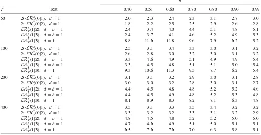
Table 1. Size simulationk=0
b
T Test 0.40 0.51 0.60 0.70 0.80 0.90 0.99
50 2s-LR2T(0|1), d=1 2.0 2.3 2.4 2.3 3.1 2.7 3.0
2s-LR2T(0|2), d=1 1.8 2.2 2.5 2.5 2.9 2.6 2.8
LR3T(1|2), d=b=1 2.4 3.4 4.0 4.4 5.1 4.8 5.1 LR3T(1|3), d=b=1 2.4 3.7 4.1 4.6 5.2 4.9 5.3 LR3
T(1|3), d=1 8.8 11.6 11.8 9.6 7.9 6.2 5.2
100 2s-LR2T(0|1), d=1 2.5 3.1 3.4 3.3 3.0 3.1 3.2
2s-LR2T(0|2), d=1 2.6 2.8 3.0 3.2 3.0 3.1 3.2
LR3T(1|2), d=b=1 3.3 4.6 4.9 5.1 4.9 4.9 5.4 LR3T(1|3), d=b=1 3.3 4.5 4.8 5.1 5.1 5.0 5.4 LR3
T(1|3), d=1 9.3 10.6 11.3 9.5 7.7 6.2 5.4
200 2s-LR2T(0|1), d=1 3.1 3.1 3.2 2.9 3.0 3.1 2.8
2s-LR2T(0|2), d=1 3.0 3.0 3.2 2.8 3.0 3.1 2.7
LR3T(1|2), d=b=1 4.4 4.5 4.8 4.8 5.2 5.2 4.6 LR3T(1|3), d=b=1 4.4 4.5 4.9 4.8 5.2 5.3 4.8 LR3
T(1|3), d=1 8.1 8.9 8.3 8.2 7.1 6.3 4.8
400 2s-LR2
T(0|1), d=1 3.5 3.1 3.3 3.5 3.4 3.2 3.2
2s-LR2T(0|2), d=1 3.3 3.2 3.2 3.3 3.1 3.2 2.9
LR3T(1|2), d=b=1 4.8 4.5 4.8 5.2 5.2 5.0 5.0 LR3T(1|3), d=b=1 4.7 4.6 4.9 5.1 5.0 5.1 5.1
LR3T(1|3), d=1 6.5 7.6 7.6 7.0 6.3 5.8 5.1
NOTES: Percentage of rejections by two-step traceLR2T(0|2) and maximum eigenvalue testLR
2
T(0|1),B=[0.5,1],Johansen’s traceLR
3
T(1|3) and maximum eigenvalueLR
3
T(1|2) tests withd=b=1 and trace testLR3
T(1|3) of Johansen and Nielsen (2012) under the null hypothesis of cointegration rankr=1 in ap=3 dimensional system withd=1,k=0. Nominal size 5%.
first cointegrating relationship and when is relatively large or small, including the caseb1=0.20 which is smaller than the lower bound ofB=[0.5,1] and allb’s. The sample size is set toT =50,100,200,400 for size simulations andT =50,100 for power analysis. For all simulations we use OxMetrics 7.00, see, Doornik and Ooms (2007) and Doornik (2009a,b), and we perform 10,000 repetitions of each experiment.
We compare the performance of the following tests discussed in this article, that is:
1. New two step procedures, that is, trace test, 2s-LR2T(0|2), and maximum eigenvalue test, 2s-LR2T(0|1),based on the FVECM for ˆβ′
⊥Xt,with the additional control ( ˆ b−1) ˜u
1t as in (16).
2. Trace and maximum eigenvalue LR tests, LR3T(1|3) and LR3T(1|2),respectively, based on the standard VECM with
d =b=1 like in Johansen (1988,1991), called Johansen’s trace and Johansen’s maximum eigenvalue tests.
3. Trace LR testLR3T(1|3) proposed by Johansen and Nielsen (2012), where estimation is restricted tod =1 and critical values are obtained from the computer program of MacKin-non and Nielsen (2014) with ML estimate ofbrounded to a decimal point.
The asymptotic distribution of Johansen’s tests in point 2 above is not justified for the data generating process (22), as they are based on a misspecified model. However, we check their performance, since they are included in most econometric packages and they are routinely used by practitioners. Similarly, Johansen and Nielsen (2012) test in point 3 is only correctly specified whenk=0,but not whenk=1,since it uses model
(17) with fractional lags Lb instead of (18) which is used to simulate data.
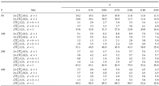
The results of our size simulations are presented in Tables 1–3. Table 1 provides the percentage of rejections under the null hypothesis of cointegration rankr =1 fork=0 and Table 2 andTable 3 for k=1 and for a=0.5 and a=0.8,
respectively. Whenk=0,the new two-step procedures are un-dersized for all sample sizes considered but improve slowly for larger samples. For moderate and large sample sizes, rejections do not change much withb,includingb=0.4. The trace LR test by Johansen and Nielsen (2012) is usually oversized, but size distortions are decreasing with sample sizeTand true value
b.Johansen’s LR tests have size close to the nominal 5% in all considered cases of moderate T, except ofb=0.4; see Table 1. Whenk=1,the two-step procedures have higher empirical size than whenk=0,being slightly oversized in smaller sam-ples, but simulated size tends to decrease withT .Whenk=1 Johansen’s tests are undersized for small values ofbin smaller samples and size distortions in these cases increase with corre-lationa.The LR test of Johansen and Nielsen (2012) heavily overrejects in all cases considered and size distortions increase with sample sizeTand correlationa,but decrease withb.
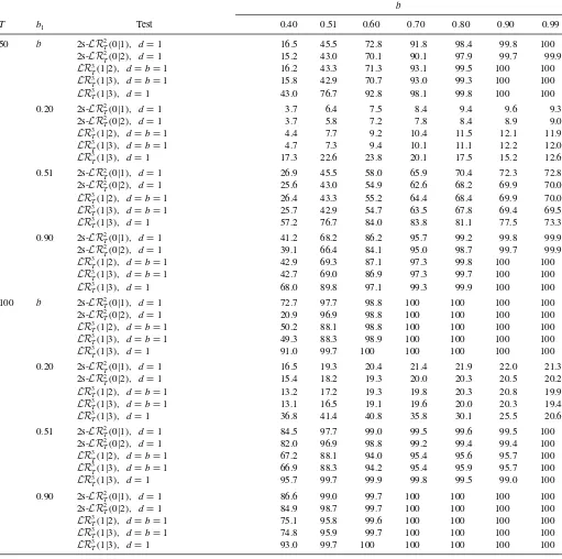
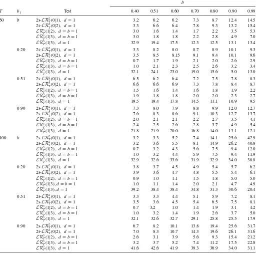
The simulated power is reported inTables 4–6forT =50 and 100.Whenk=0,seeTable 4, all procedures have very good power for all sample sizesTand all true values ofb, b1,except
b1=0.20,which is very difficult to detect whenT =50.The power of all tests is increasing with sample sizeT , b,andb1, two-step method doing marginally better for smallband/orb1, while Johansen tests do better whenT =50 andb1≥0.9,since this case is closer to the unit root model assumed by these tests.
Table 2. Size simulationk=1, a=0.5
b
T Test 0.40 0.51 0.60 0.70 0.80 0.90 0.99
50 2s-LR2T(0|1), d=1 7.2 7.2 8.2 8.7 9.9 10.3 10.7
2s-LR2T(0|2), d=1 7.4 7.1 8.4 8.5 9.8 10.6 10.6
LR3
T(1|2), d=b=1 1.5 1.5 2.1 2.6 3.4 4.2 5.0
LR3T(1|3), d=b=1 1.7 1.7 2.6 3.1 3.8 4.6 5.3
LR3T(1|3), d=1 11.5 13.3 13.1 11.5 9.6 8.6 7.1
100 2s-LR2T(0|1), d=1 4.6 5.2 6.0 6.6 6.4 7.2 7.2
2s-LR2T(0|2), d=1 4.2 5.1 5.8 6.7 6.3 7.0 7.1
LR3
T(1|2), d=b=1 1.4 2.1 3.0 4.0 4.7 5.5 6.3
LR3T(1|3), d=b=1 1.5 2.2 3.1 4.5 4.6 5.7 6.2
LR3T(1|3), d=1 17.7 20.6 22.6 18.8 14.9 11.5 8.2
200 2s-LR2T(0|1), d=1 4.3 5.0 5.7 5.5 4.9 4.8 4.6
2s-LR2T(0|2), d=1 4.2 4.8 5.2 5.3 4.8 4.8 4.5
LR3T(1|2), d=b=1 2.1 3.2 4.4 5.4 5.4 5.4 5.1
LR3T(1|3), d=b=1 2.2 3.3 4.4 5.1 5.5 5.5 5.3
LR3T(1|3), d=1 36.7 41.8 38.5 29.4 18.5 10.4 6.3
400 2s-LR2T(0|1), d=1 4.7 4.6 4.4 4.5 4.1 4.0 3.9
2s-LR2T(0|2), d=1 4.5 4.5 4.4 4.3 3.6 3.6 3.9
LR3T(1|2), d=b=1 2.0 4.4 5.1 5.3 5.2 5.2 5.2
LR3T(1|3), d=b=1 2.0 4.5 5.0 5.4 5.2 5.2 5.4
LR3T(1|3), d=1 57.9 67.3 55.8 36.8 17.0 8.3 5.7
NOTES: Percentage of rejections by two-step traceLR2
T(0|2) and maximum eigenvalue testLR2T(0|1),B=[0.5,1],Johansen’s traceLR3T(1|3) and maximum eigenvalueLR3T(1|2) tests withd=b=1 and trace testLR3T(1|3) of Johansen and Nielsen (2012) under the null hypothesis of cointegration rankr=1 in ap=3 dimensional system withd=1,k=1, a=0.5.Nominal size 5%.
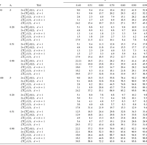
Whenk=1 all procedures are much less powerful than fork= 0,especially for the larger value of the autoregressive coefficient a and smallb; seeTable 5 andTable 6. However, still power increases with sample sizeT,b,andb1for all methods.
Two-step procedures are noticeably more powerful than Johansen tests except of the cases close tob=b1=1 in sampleT =100. The LR test of Johansen and Nielsen (2012) has largest power among all in many parameter combinations, but it is not relevant
Table 3. Size simulationk=1, a=0.8
b
T Test 0.4 0.51 0.60 0.70 0.80 0.90 0.99
50 2s-LR2
T(0|1), d=1 10.2 10.1 10.9 10.6 11.6 11.0 11.5
2s-LR2T(0|2), d=1 10.8 10.1 10.9 10.9 11.7 11.4 12.0
LR3T(1|2), d=b=1 3.1 2.9 2.7 3.0 3.3 3.4 4.1
LR3
T(1|3), d=b=1 3.7 3.3 3.2 3.7 3.8 4.1 4.9 LR3T(1|3), d=1 33.6 32.9 31.5 27.0 22.6 20.6 18.4
100 2s-LR2T(0|1), d=1 5.1 5.5 6.2 6.6 6.9 7.9 7.8
2s-LR2T(0|2), d=1 5.3 5.5 6.4 6.9 7.0 7.7 7.4
LR3T(1|2), d=b=1 1.2 1.3 1.5 2.1 2.6 3.6 5.0
LR3
T(1|3), d=b=1 1.6 1.5 1.9 2.4 2.9 4.0 5.3 LR3T(1|3), d=1 51.1 49.5 49.0 45.9 43.3 38.9 25.8
200 2s-LR2T(0|1), d=1 3.7 4.2 4.7 5.4 5.7 5.4 5.7
2s-LR2T(0|2), d=1 3.6 4.2 4.5 5.2 5.7 5.4 5.7
LR3T(1|2), d=b=1 0.8 1.1 1.8 2.6 4.2 5.3 5.8
LR3
T(1|3), d=b=1 1.0 1.4 1.9 2.9 4.7 5.4 6.0 LR3T(1|3), d=1 83.2 83.1 83.9 82.9 79.3 53.4 29.8
400 2s-LR2T(0|1), d=1 3.7 4.0 4.6 5.0 4.4 4.5 4.3
2s-LR2T(0|2), d=1 3.7 3.8 4.6 4.5 4.3 4.5 4.5
LR3T(1|2), d=b=1 1.2 2.0 3.5 4.8 5.2 5.8 5.8
LR3T(1|3), d=b=1 1.3 2.2 3.7 5.0 5.3 5.8 5.9
LR3T(1|3), d=1 99.3 99.3 99.5 99.3 90.7 52.4 25.6
NOTES: Percentage of rejections by two-step traceLR2
T(0|2) and maximum eigenvalue testLR
2
T(0|1),B=[0.5,1],Johansen’s traceLR
3
T(1|3) and maximum eigenvalueLR
3
T(1|2) tests withd=b=1 and trace testLR3
T(1|3) of Johansen and Nielsen (2012) under the null hypothesis of cointegration rankr=1 in ap=3 dimensional system withd=1,k=1, a=0.8.Nominal size 5%.
Table 4. Power simulationk=0
b
T b1 Test 0.40 0.51 0.60 0.70 0.80 0.90 0.99
50 b 2s-LR2T(0|1), d=1 16.5 45.5 72.8 91.8 98.4 99.8 100 2s-LR2T(0|2), d=1 15.2 43.0 70.1 90.1 97.9 99.7 99.9 LR3T(1|2), d=b=1 16.2 43.3 71.3 93.1 99.5 100 100 LR3T(1|3), d=b=1 15.8 42.9 70.7 93.0 99.3 100 100 LR3
T(1|3), d=1 43.0 76.7 92.8 98.1 99.8 100 100
0.20 2s-LR2T(0|1), d=1 3.7 6.4 7.5 8.4 9.4 9.6 9.3 2s-LR2T(0|2), d=1 3.7 5.8 7.2 7.8 8.4 8.9 9.0 LR3T(1|2), d=b=1 4.4 7.7 9.2 10.4 11.5 12.1 11.9 LR3T(1|3), d=b=1 4.7 7.3 9.4 10.1 11.1 12.2 12.0 LR3
T(1|3), d=1 17.3 22.6 23.8 20.1 17.5 15.2 12.6
0.51 2s-LR2T(0|1), d=1 26.9 45.5 58.0 65.9 70.4 72.3 72.8 2s-LR2T(0|2), d=1 25.6 43.0 54.9 62.6 68.2 69.9 70.0 LR3T(1|2), d=b=1 26.4 43.3 55.2 64.4 68.4 69.9 70.0 LR3T(1|3), d=b=1 25.7 42.9 54.7 63.5 67.8 69.4 69.5 LR3
T(1|3), d=1 57.2 76.7 84.0 83.8 81.1 77.5 73.3
0.90 2s-LR2
T(0|1), d=1 41.2 68.2 86.2 95.7 99.2 99.8 99.9
2s-LR2T(0|2), d=1 39.1 66.4 84.1 95.0 98.7 99.7 99.9 LR3T(1|2), d=b=1 42.9 69.3 87.1 97.3 99.8 100 100 LR3T(1|3), d=b=1 42.7 69.0 86.9 97.3 99.7 100 100 LR3T(1|3), d=1 68.0 89.8 97.1 99.3 99.9 100 100 100 b 2s-LR2
T(0|1), d=1 72.7 97.7 98.8 100 100 100 100
2s-LR2T(0|2), d=1 20.9 96.9 98.8 100 100 100 100 LR3T(1|2), d=b=1 50.2 88.1 98.8 100 100 100 100 LR3T(1|3), d=b=1 49.3 88.3 98.9 100 100 100 100 LR3T(1|3), d=1 91.0 99.7 100 100 100 100 100 0.20 2s-LR2
T(0|1), d=1 16.5 19.3 20.4 21.4 21.9 22.0 21.3
2s-LR2T(0|2), d=1 15.4 18.2 19.3 20.0 20.3 20.5 20.2 LR3T(1|2), d=b=1 13.2 17.2 19.3 19.8 20.3 20.8 19.9 LR3T(1|3), d=b=1 13.1 16.5 19.1 19.6 20.0 20.3 19.4 LR3T(1|3), d=1 36.8 41.4 40.8 35.8 30.1 25.5 20.6 0.51 2s-LR2
T(0|1), d=1 84.5 97.7 99.0 99.5 99.6 99.5 100
2s-LR2T(0|2), d=1 82.0 96.9 98.8 99.2 99.4 99.4 100 LR3T(1|2), d=b=1 67.2 88.1 94.0 95.4 95.6 95.7 100 LR3
T(1|3), d=b=1 66.9 88.3 94.2 95.4 95.9 95.7 100 LR3T(1|3), d=1 95.7 99.7 99.9 99.8 99.5 99.0 100 0.90 2s-LR2
T(0|1), d=1 86.6 99.0 99.7 100 100 100 100
2s-LR2T(0|2), d=1 84.9 98.7 99.7 100 100 100 100 LR3T(1|2), d=b=1 75.1 95.8 99.6 100 100 100 100 LR3
T(1|3), d=b=1 74.8 95.9 99.7 100 100 100 100 LR3T(1|3), d=1 93.0 99.7 100 100 100 100 100
NOTES: Percentage of rejections by two step traceLR2T(0|2) and maximum eigenvalue testLR
2
T(0|1),B=[0.5,1],Johansen’s traceLR
3
T(1|3) and maximum eigenvalueLR
3
T(1|2) tests withd=b=1 and trace testLR3
T(1|3) of Johansen and Nielsen (2012) under the alternative hypothesis of cointegration rankr=2 inp=3 dimensional system withd=1, k=0 and second cointegrating relationship with the memoryb1=b,0.20,0.51, or 0.9. Nominal size 5%.
as this test does not keep the size in this experiment. To sum up, two-step rank tests have a similar behavior to the one-step LR test whend=b≈1, however they seem to be more powerful whenband/orb1are small, being able to exploit the differences betweenbandb1or (b, b1) andd,which are fixed in Johansen (1998) and Johansen and Nielsen (2012) methodologies.
6. ANALYSIS OF THE TERM STRUCTURE OF THE INTEREST RATES
To illustrate the empirical relevance of the described method-ology we reconsider the analysis of the term structure of the
interest rates by Iacone (2009). There has been a lot of interest in this issue in the current literature; see, for example, Chen and Hurvich (2003) and Nielsen (2010).
As argued in Iacone (2009), a good model of the term struc-ture of the interest rates is needed to measure the effects of the monetary policy and to price financial assets. It is an important tool for policy evaluation since the Federal Reserve operates in just one market, the one with contracts with very short maturity. Therefore, it is necessary to model the conduction of the mone-tary policy impulses to the rates of contracts with longer maturi-ties. Modeling the interactions across rates is also important for
Table 5. Power simulationk=1, a=0.5
b
T b1 Test 0.40 0.51 0.60 0.70 0.80 0.90 0.99
50 b 2s-LR2T(0|1), d=1 9.0 9.4 13.4 19.4 29.2 41.9 52.8 2s-LR2T(0|2), d=1 9.1 9.8 13.7 20.2 29.3 42.2 52.2 LR3
T(1|2), d=b=1 2.8 2.3 4.0 7.9 15.1 28.2 44.5 LR3T(1|3), d=b=1 3.1 2.7 4.5 8.9 16.5 29.2 45.0 LR3T(1|3), d=1 24.2 15.4 19.7 23.3 27.1 35.7 45.2 0.20 2s-LR2T(0|1), d=1 5.1 6.6 8.2 8.3 9.8 10.9 11.2 2s-LR2T(0|2), d=1 4.8 6.9 8.1 8.6 9.7 10.8 11.0 LR3
T(1|2), d=b=1 1.3 1.4 1.8 2.3 3.3 3.9 4.5 LR3T(1|3), d=b=1 1.5 1.6 2.0 2.7 3.3 4.2 4.9 LR3T(1|3), d=1 17.9 11.5 12.1 10.1 8.4 7.6 6.4 0.51 2s-LR2T(0|1), d=1 5.1 9.4 11.3 12.8 15.3 17.4 17.6 2s-LR2T(0|2), d=1 4.8 9.8 11.6 13.4 15.5 17.7 17.1 LR3T(1|2), d=b=1 1.3 2.3 2.9 4.0 5.5 7.3 9.1 LR3T(1|3), d=b=1 1.5 2.7 3.3 4.9 5.9 8.4 9.7 LR3T(1|3), d=1 17.9 15.4 16.5 15.2 12.7 12.3 10.8 0.90 2s-LR2T(0|1), d=1 22.21 18.5 23.1 28.2 35.1 41.4 45.3 2s-LR2T(0|2), d=1 21.11 19.0 23.6 29.1 35.9 41.6 45.5 LR3T(1|2), d=b=1 16.0 7.7 10.5 14.7 20.4 28.2 34.6 LR3T(1|3), d=b=1 16.2 8.3 11.4 16.1 21.6 29.1 35.9 LR3T(1|3), d=1 39.5 27.7 32.6 33.8 33.9 35.7 36.5 100 b 2s-LR2T(0|1), d=1 9.0 18.5 33.5 55.6 78.4 92.2 96.5 2s-LR2T(0|2), d=1 9.1 18.6 32.6 53.8 76.5 90.9 95.7 LR3T(1|2), d=b=1 2.8 8.2 20.1 44.5 74.6 94.8 99.3 LR3T(1|3), d=b=1 3.1 8.9 20.8 43.7 73.8 93.6 99.1 LR3T(1|3), d=1 24.2 37.2 53.1 68.9 85.2 95.6 99.1 0.20 2s-LR2T(0|1), d=1 5.1 6.0 7.6 8.6 9.7 10.2 9.6
2s-LR2
T(0|2), d=1 5.0 6.1 7.3 8.4 9.6 10.1 9.3 LR3T(1|2), d=b=1 3.4 4.1 4.8 5.7 6.3 6.7 6.2 LR3T(1|3), d=b=1 3.6 4.0 4.6 5.7 6.3 6.8 6.1 LR3T(1|3), d=1 17.8 31.4 21.9 19.7 15.3 12.9 9.4 0.51 2s-LR2T(0|1), d=1 12.5 18.5 24.4 29.6 32.6 34.5 33.4
2s-LR2
T(0|2), d=1 12.9 18.6 24.1 29.6 31.9 33.6 32.6 LR3T(1|2), d=b=1 4.9 8.2 13.3 18.5 23.8 28.8 29.1 LR3T(1|3), d=b=1 5.4 8.7 13.7 19.1 23.8 28.6 28.9 LR3T(1|3), d=1 29.3 37.2 43.4 42.6 39.1 37.0 31.0 0.90 2s-LR2T(0|1), d=1 22.2 37.2 53.9 70.9 85.2 92.2 93.9
2s-LR2
T(0|2), d=1 22.1 36.8 52.3 69.3 83.8 90.9 93.0 LR3T(1|2), d=b=1 16.0 28.4 44.6 66.7 84.6 94.8 97.2 LR3T(1|3), d=b=1 16.2 29.3 44.6 65.5 83.8 93.6 96.6 LR3
T(1|3), d=1 39.5 56.8 72.2 83.9 91.4 95.6 96.6 NOTES: Percentage of rejections by two step traceLR2
T(0|2) and maximum eigenvalue testLR2T(0|1),B=[0.5,1],Johansen’s traceLR3T(1|3) and maximum eigenvalueLR3T(1|2) tests withd=b=1 and trace testLR3T(1|3) of Johansen and Nielsen (2012) under the alternative hypothesis of cointegration rankr=2 inp=3 dimensional system withd=1, k=1, a=0.5,, and second cointegrating relationship with the memoryb1=b,0.20,0.51 or 0.9.Nominal size 5%.
the economic agents to forecast the effects of future monetary policy decisions on the price of financial assets. Soderlind and Svensson (1997) discussed a practical example of how to extract the market’s expectations on future policy rates from a given term structure, and how to use them to price financial instruments.
Cointegration has an appealing feature in the analysis of the term structure, because it makes possible to distinguish the high persistence of shocks to interest rates from the much lower persistence of shocks to the spreads. Standard cointegration in
the context of modeling a vector of U.S. dollar interest rates has been considered by Hall, Anderson, and Granger (1992), Engsted and Tangaard (1994), and Dominguez and Novales (2000).
However, it has been argued that the unit root model for the interest rates is often incompatible with monetary and finance theories, because it may imply a unit root model for the expected inflation rate as well. This is the case, for example, if the real interest rate is constant in the long run, or if the central bank sets the interest rate using a linear reaction function like the
Table 6. Power simulationk=1, a=0.8
b
T b1 Test 0.40 0.51 0.60 0.70 0.80 0.90 0.99
50 b 2s-LR2T(0|1), d=1 3.2 6.2 6.2 7.3 8.7 12.4 14.5
2s-LR2T(0|2), d=1 3.3 6.6 6.4 7.8 9.3 13.2 15.4 LR3T(1|2), d=b=1 3.0 1.6 1.4 1.7 2.2 3.5 5.3 LR3T(1|3), d=b=1 3.0 1.8 1.8 2.2 2.8 4.9 7.0 LR3
T(1|3), d=1 32.9 19.4 17.5 12.3 12.5 13.1 13.4
0.20 2s-LR2T(0|1), d=1 3.3 8.2 8.0 8.7 8.9 10.1 9.3 2s-LR2T(0|2), d=1 3.5 8.5 8.15 9.1 9.4 10.1 9.6 LR3T(1|2), d=b=1 0.7 1.7 1.9 2.1 2.0 2.6 2.9 LR3T(1|3), d=b=1 1.0 2.1 2.3 2.5 2.6 3.2 3.4 LR3
T(1|3), d=1 32.1 24.1 23.0 19.0 15.6 5.0 13.0
0.51 2s-LR2T(0|1), d=1 6.5 6.2 6.4 7.2 7.5 7.8 8.3 2s-LR2T(0|2), d=1 6.6 6.6 6.9 7.3 7.8 8.4 8.7 LR3T(1|2), d=b=1 1.5 1.6 1.4 1.6 1.8 1.9 2.2 LR3T(1|3), d=b=1 1.9 1.8 1.8 2.0 2.0 2.3 2.7 LR3
T(1|3), d=1 19.5 19.4 17.8 14.5 11.1 10.9 9.5
0.90 2s-LR2
T(0|1), d=1 7.3 8.0 7.9 8.8 9.9 12.0 12.7
2s-LR2T(0|2), d=1 7.6 8.3 8.6 9.1 10.3 12.7 13.7 LR3T(1|2), d=b=1 2.0 2.1 2.1 2.2 2.7 3.5 4.1 LR3T(1|3), d=b=1 2.4 2.5 2.6 2.8 3.7 4.9 5.4 LR3T(1|3), d=1 21.8 21.9 20.0 16.8 14.0 13.1 12.1 100 b 2s-LR2
T(0|1), d=1 3.2 3.3 5.2 7.4 14.1 25.6 42.9
2s-LR2T(0|2), d=1 3.2 3.6 5.5 8.1 14.9 26.2 40.8 LR3T(1|2), d=b=1 0.7 3.2 4.3 5.6 7.5 9.4 12.0 LR3T(1|3), d=b=1 1.0 3.2 4.4 5.9 7.5 9.4 11.9 LR3T(1|3), d=1 32.9 32.6 33.6 31.9 32.9 34.0 38.8 0.20 2s-LR2
T(0|1), d=1 3.8 3.7 4.5 4.9 5.4 5.7 6.2
2s-LR2T(0|2), d=1 3.9 3.6 4.7 4.8 5.5 5.4 6.1 LR3T(1|2), d=b=1 0.9 1.0 1.1 1.5 1.8 5.0 5.0 LR3T(1|3), d=b=1 1.0 1.1 1.4 2.0 2.1 4.7 4.9 LR3T(1|3), d=1 39.2 38.4 38.4 34.8 31.3 30.6 20.4 0.51 2s-LR2
T(0|1), d=1 3.3 3.3 4.4 5.1 5.9 7.2 8.1
2s-LR2T(0|2), d=1 3.5 3.6 4.5 5.4 6.5 7.5 8.1 LR3T(1|2), d=b=1 0.7 3,2 1.0 1.4 1.9 3.1 4.2 LR3
T(1|3), d=b=1 1.0 3.2 1.4 1.9 2.6 3.7 5.0 LR3T(1|3), d=1 32.1 32.6 32.7 29.1 25.8 25.5 17.9 0.90 2s-LR2
T(0|1), d=1 6.7 8.2 10.1 13.8 19.4 25.6 31.7
2s-LR2T(0|2), d=1 7.0 8.3 10.7 14.3 19.6 26.1 31.6 LR3T(1|2), d=b=1 2.6 3.1 3.9 5.6 9.3 15.4 21.2 LR3
T(1|3), d=b=1 3.2 3.7 5.2 7.4 11.2 17.5 22.8 LR3T(1|3), d=1 41.6 42.6 41.9 39.3 36.9 34.0 31.1
NOTES: Percentage of rejections by two-step traceLR2T(0|2) and maximum eigenvalue testLR
2
T(0|1),B=[0.5,1],Johansen’s traceLR
3
T(1|3) and maximum eigenvalueLR
3
T(1|2) tests withd=b=1 and trace testLR3
T(1|3) of Johansen and Nielsen (2012) under the alternative hypothesis of cointegration rankr=2 inp=3 dimensional system withd=1, k=1, a=0.8,and second cointegrating relationship with the memoryb1=b,0.20,0.51, or 0.9. Nominal size 5%.
ones described by Taylor (1993) or by Svensson (1997). Such a strong persistence is hardly acceptable, because it implies that the central bank does not stabilize inflation.
We can allow for fractional cointegration instead. It permits to combine high persistence with mean reversion in the long run, and it maintains the possibility of the presence of a common stochastic terms in multivariate processes. Fractional integration may be motivated as the result of occasional breaks in an other-wise weakly autocorrelated process. This interpretation seems particularly appealing when modeling the interest rates because
changes to the discount rate are infrequent. Granger and Hyoung (2004) showed that fractional integration and occasional breaks may in practice be indistinguishable and, following a comment by Diebold and Inoue (2001), adopting fractional integration in a model may result in good forecasts.
We analyze the behavior of the U.S. dollar interest rates with maturities of 1, 3, and 6 months (the London InterBank Of-fered Rate LIBOR) over the period 01/1963-04/2006. The data come from DataStream with identification codes being, respec-tively, USI60LDC, USI60LDD, USI60LDE. LIBOR is not
Table 7. Rank tests statistics underH0:r=1, d=dˆ=0.88
LR test 2-step Johansen J-N
max lambda 19.04 53.8 –
trace 19.04 54.5 30.7
Table 8. 5% Critical values of rank tests underH0:r=1,p=3
2-step 2-step
LR test (B= [0.5,1]) (B= [0.5,0.88]) Johansen J-N
max lambda 11.72 11.02 11.23 –
trace 12.84 12.13 12.32 10.95
fected by any regulation imposed by the central bank, and thus it is a typical measure of the cost of funds in U.S. dollars. For this dataset, Iacone (2009) found evidence that the three considered series share the same order of integration with esti-mated ˆd =0.88. The test of Robinson and Yajima (2002) and local Whittle procedure of Robinson (1995) have been used to obtain this result. Iacone (2009) also concluded the frac-tional cointegration with rankr=2 in this system using proce-dures in Phillips and Ouliaris (1988) and Robinson and Yajima (2002).
However the integration order of the cointegrating residuals of two relations found by Iacone (2009) differ significantly, and the transmission of impulses is slower the longer distance (in maturity) from the market, where the Federal Reserve is directly present, so a model that allows differentb’s would be appro-priate for this example. Łasak (2008) analyzed three bivariate systems and has not imposed the assumption that both cointe-gration relationships share the same memory. The methodology developed in this article enables us to test the rank directly in the 3-variate system (1) without imposing such assumption, as we pursue.
We consider the basic version of the model presented in Sec-tion 3, as it seems to be a right choice looking at PACF of the processes. We have tested the existence of the breaks in levels of considered series using the test of Sibbertsen and Kruse (2009) and it has indicated no breaks in the series. All the tests con-sidered in Section 5 have been computed and all confirm that this system is cointegrated with rank 2. The values of the test statistics when testing rankr =1 are presented inTable 7.
In Table 8 we provide the 5% critical values for two-step tests when d =0.88 and B=[0.5,0.88], compared to those whend =1 andB=[0.5,1].The critical values ford <1 are smaller than those ford =1, and in general, using the latter for situations whend <1 would lead to a conservative inference. In any case, the tests statistics in Table 7 are significant at the 5% level even using the conservative critical values ford =1.
We also estimate the cointegration vectors on the basis of all considered models, including the VECM withd =b=1 and the FVECM (1) withd =dˆ=0.88 imposed,which is justified by Corollary 1. The first cointegration relationship is common to all procedures, but the second one can be different. When we focus on the two-step procedure proposed in Section 3, the esti-mate of the second cointegrating relationshipβ1is found accord-ing to the formula ˆβ1=β⊥′β
∗
1,whereβ1∗ comes directly from
Table 9. Estimates ofbandb1,d=dˆ=0.88.
1st step ( ˆb) 2nd step ( ˆb1) J-N
ˆ
b 0.81 0.88 0.83
solving the eigenvalue problem (2) constructed on the basis of the transformed model (16). It turns out that the outcomes of all the procedures imply the same cointegrating space spanned by
ˆ
βnorm=
⎡
⎣
1 1
−0.98 0 0 −0.96
⎤
⎦.
The cointegrating parameters are very close to −1, so the spreads can be computed asst(j) =i
(j) t −i
(1)
t , j=3,6.Iacone (2009) estimated the orders of integration of these spreads using the local Whittle estimator of Robinson (1995) to be
s(tj) ∼ I(dj−bj), s (3)
t ∼I(0.34), ands (6)
t ∼I(0.47) and re-jected the hypothesis that these orders are the same. Therefore, the rank estimation methodology developed in this article is suitable for this example, as it takes into account the possibility that the persistence of the cointegration relationships differ. However, when we estimated the FVECM using ML our results do not confirm that the spreads are persistent.
Looking at the estimates of the order of cointegrationb in Table 9 we might conclude that the spreads seem to behave asI(0) processes, so the evidence supporting the expectation hypothesis can be found in the multivariate case if the analysis does not restrict all the cointegration relationships to share the same memory.
7. CONCLUSIONS
In this article we have proposed a new procedure, based on sequential two-step LR tests, to establish the cointegration rank in a fractional system. The main novelty is that it allows the cointegrating relationships under the alternative to have differ-ent memory compared to the null ones. It only needs a small modification of the model estimated in the second step. The asymptotic distributions of the test statistics are the same as for the no-cointegration testing, so the set of simulations required to approximate the critical values is reduced, which can be seen as an advantage for empirical work. We have investigated the per-formance of our procedure in finite samples and have compared it with the LR trace test of Johansen and Nielsen (2012) and with Johansen’s LR trace and maximum eigenvalue tests. We have found that our tests control size and have an advantage in terms of power to detect extra cointegrating relationships in situations when the memories of the cointegration relations differ or are relatively small.
ACKNOWLEDGMENTS
The authors are very grateful to the Associate Editor and two referees, Niels Haldrup, Lennart Hoogerheide, Søren Jo-hansen, Siem Jan Koopman, Morten Ørregaard Nielsen, and participants at various seminars and conferences for helpful comments and suggestions. Research support from the Spanish
Plan Nacional de I+D+I (ECO2012-31748) is gratefully ac-knowledged. The first author also acknowledges support from CREATES - Center for Research in Econometric Analysis of Time Series (DNRF78), funded by the Danish National Re-search Foundation and the Tinbergen Institute in the Nether-lands.
APPENDIX
Proof of Theorem 1. We demonstrate first that replacingβ⊥by ˆβ⊥
makes no difference asymptotically in the two-step LR test statistics. LR tests statistics depend on properly normalized sample moments of dependent and independent variables in the regression model (16); see (2).The result follows from Theorem 1 in Łasak (2010), after controlling for the projection on (b
+−1)u1tas in Lemma 10.3 in
Jo-hansen (1995), using the representation (14) for the dependent variable
V0t =β⊥′dXt.
The second term on the right-hand side of (23) is
T−b1 Using the same ideas it can be shown that
T−2b1
exploiting (103) and (102), respectively, in Lemma A.9 in Johansen and Nielsen (2012), so that the estimation ofβ⊥in the first step has no
impact on the asymptotic distribution of the test statistics. We next show that replacing (b
+−1)u1t by (
that, it is enough to consider the differences
T−b1
b1 as in Robinson and Hualde (2003, Proposition 9), expanding
(b
totically stationary process, and the superconsistency of ˆβ.Finally, the analysis of (25) beingop(1) is simpler because it does not depend on
b1andutis iid.
Then to show the validity of the correction introduced in regression (16), it is only necessary to observe that the vectorutis just a rotation
of the vectorεt,so all previous approximations and bounds can be used
similarly.
Proof of Corollary 1. We have to additionally show that terms like
T−b1
from a similar analysis as that of the first term in (26), writing this difference as
⊥Xt, and then using uniform bounds for the
corresponding sample moments on (derivatives of) fractionally
inte-grated processes.
Proof of Theorem 2. The proof follows the lines of the proof of The-orem 1, since the additional lagsdX
t−j, j=1, . . . , kin regression
(20) pose no additional problem compared to the projection of ˆV0tand
ˆ
V1t(b1) on (+bˆ −1) ˆu1t, because the former are observed andI(0).
[Received March 2013. Revised May 2014.]
REFERENCES
Avarucci, M., and Velasco, C. (2009), “A Wald Test for the Cointegration Rank in Nonstationary Fractional Systems,”Journal of Econometrics, 151, 178– 189. [241,242,245]
Breitung, J., and Hassler, U. (2002), “Inference on the Cointegration Rank in Fractionally Integrated Processes,”Journal of Econometrics, 110, 167–185. [241]
Chen, W., and Hurvich, C. (2003), “Semiparametric Estimation of Multivariate Fractional Cointegration,”Journal of American Statistical Association, 98, 629–642. [241,249]
——— (2006), “Semiparametric Estimation of Fractional Cointegrating Sub-spaces,”The Annals of Statistics, 34, 2939–2979. [241]
Davies, R. B. (1977), “Hypothesis Testing When a Nuisance is Present Only Under the Alternative,”Biometrika, 64, 247–254. [243]
Diebold, F. X., and Inoue, A. (2001), “Long Memory and Regime Switching,”
Journal of Econometrics, 105, 131–159. [251]
Dominguez, E., and Novales, A. (2000), “Testing the Expectations Hypothesis in Eurodeposits,”Journal of International Money and Finance, 19, 713–736. [250]
Doornik, J. A. (2009a),An Introduction to OxMetrics(Vol. 6), London: Tim-berlake Consultants Press. [247]
——— (2009b),An Object-Oriented Matrix Language Ox 6, London: Timber-lake Consultants Press. [247]
Doornik, J. A., and Ooms, M. (2007),Introduction to Ox: An Object-Oriented Matrix Language, London: Timberlake Consultants Press. [247]
Engsted, T., and Tangaard, C. (1994), “Cointegration and the U.S. Term Struc-ture,”Journal of Banking and Finance, 18, 167–181. [250]
Gil-Ala˜na, L. A. (2003), “Testing of Fractional Cointegration in Macroeconomic Time Series,”Oxford Bulletin of Economics and Statistics, 65, 517–529. [241]
Granger, C. W. J. (1986), “Developments in the Study of Cointegrated Eco-nomic Variables,”Oxford Bulletin of Economics and Statistics, 48, 213– 228. [242]
Granger, C. W. J., and Hyung, N. (2004), “Occasional Structural Breaks and Long Memory With an Application to the S&P 500 Absolute Stock Returns,”
Journal of Empirical Finance, 11, 399–421. [251]
Hall, A. D., Anderson, H. M., and Granger, C. W. J. (1992), “A Cointegration Analysis of Treasury Bill Yields,”The Review of Economics and Statistics, 74, 116–126. [250]
Hansen, B. E. (1996), “Inference When a Nuisance Parameter is Not Identified Under the Null Hypothesis,”Econometrica, 64, 413–430. [243]
Hualde, J., and Velasco, C. (2008), “Distribution-Free Tests of Fractional Coin-tegration, “Econometric Theory, 24, 216–255. [241]
Iacone, F. (2009), “A Semiparametric Analysis of the Term Structure of the US Interest Rates,”Oxford Bulletin of Economics and Statistics, 71, 475–490. [249,252]
Johansen, S. (1988), “Statistical Analysis of Cointegration Vectors,”Journal of Economic Dynamics and Control, 12, 231–254. [241,242,247]
——— (1991), “Estimation and Hypothesis Testing of Cointegration Vectors in Gaussian Vector Autoregressive Models,”Econometrica, 59, 1551–1580. [241,242,247]
——— (1995), Likelihood-Based Inference in Cointegrated Vector Auto-Regressive Models, Oxford, UK: Oxford University Press. [253]
——— (2008), “A Representation Theory for a Class of Vector Autoregres-sive Models for Fractional Processes,”Econometric Theory, 24, 651–676. [242,244,245]
——— (2009), “Representation of Cointegrated Autoregressive Processes With Application to Fractional Cointegration,”Econometric Reviews, 28, 121– 145. [242,245]
Johansen, S., and Nielsen, M. Ø. (2012), “Likelihood Inference for a Fractionally Cointegrated Vector Autoregressive Model,”Econometrica, 80, 2667–2732. [241,242,243,244,245,247,252,253]
Łasak, K. (2008), “Maximum Likelihood Estimation of Fractionally Cointe-grated Systems,” CREATES Research Paper 2008-53. [241,242,252] ——— (2010), “Likelihood Based Testing for No Fractional Cointegration,”
Journal of Econometrics, 158, 67–77. [241,242,243,244,253]
MacKinnon, J. G., and Nielsen, M. Ø. (2014), “Numerical Distribution Func-tions of Fractional Unit Root and Cointegration Tests,”Journal of Applied Econometrics, 29, 161–171. [243,247]
Marinucci, D., and Robinson, P. M. (2001), “Semiparametric Fractional Coin-tegration Analysis,”Journal of Econometrics, 105, 225–247. [241] Marmol, F., and Velasco, C. (2004), “Consistent Testing of Cointegrating
Rela-tionships,”Econometrica, 72, 1809–1844. [241]
Nielsen, M. Ø. (2004), “Optimal Residual-Based Tests for Fractional Cointe-gration and Exchange Rate Dynamics,”Journal of Business and Economic Statistics, 22, 331–345. [241]
——— (2005), “Multivariate Lagrange Multiplier Tests for Fractional Integra-tion,”Journal of Financial Econometrics, 3, 372–398. [241]
———- (2010), “Nonparametric Cointegration Analysis of Fractional Systems With Unknown Integration Orders,”Journal of Econometrics, 155, 170– 187. [249]
Nielsen, M. Ø., and Shimotsu, K. (2007), “Determining the Cointegrating Rank in Nonstationary Fractional Systems by Exact Local Whittle Approach,”
Journal of Econometrics, 141, 574–596. [241]
Phillips, P. C. B., and Ouliaris, S. (1988), “Testing for Cointegration Using Prin-cipal Component Measures,”Journal of Economic Dynamics and Control, 12, 205–230. [252]
Robinson, P. M. (1995), “Gaussian Semiparametric Estimation of Long Range Dependence,”The Annals of Statistics, 23, 1630–1661. [252]
——— (2008), “Diagnostic Testing for Cointegration,”Journal of Economet-rics, 143, 206–225. [241]
Robinson, P. M., and Hualde, J. (2003), “Cointegration in Fractional Sys-tems With Unknown Integration Orders,”Econometrica, 71, 1727–1766. [241,245,253]
Robinson, P. M., and Yajima, Y. (2002), “Determination of Cointegrating Rank in Fractional Systems,”Journal of Econometrics, 106, 217–241. [241,252] Sibbertsen, P., and Kruse, R. (2009), “Testing for a Break in Persistence Under Long-Range Dependencies,”Journal of Time Series Analysis, 30, 263–285. [252]
Soderlind, P., and Svensson, L. (1997), “New Techniques to Extract Market Expectations From Financial Instruments,”Journal of Monetary Economics, 40, 383–429. [250]
Svensson, L. E. O. (1997), “Inflation Forecast Targeting: Implementing and Monitoring Inflation Targets,”European Economic Review, 41, 1111–1146. [251]
Taylor, J. B. (1993), “Discretion Versus Policy Rules in Practice,” Carnegie-Rochester Conference Series on Public Policy, 39, 195–214. [251]