El e c t ro n ic
Jo ur
n a l o
f P
r o
b a b il i t y
Vol. 13 (2008), Paper no. 65, pages 1980–2013. Journal URL
http://www.math.washington.edu/~ejpecp/
Glauber dynamics on nonamenable graphs:
boundary conditions and mixing time
Alessandra Bianchi
Weierstrass Institute for Applied Analysis and Stochastics
Mohrenstrasse 39, 10117 Berlin, Germany
Email: [email protected]
Abstract
We study the stochastic Ising model on finite graphs with nvertices and bounded degree and analyze the effect of boundary conditions on the mixing time. We show that for all low enough temperatures, the spectral gap of the dynamics with(+)-boundary condition on a class of non-amenable graphs, is strictly positive uniformly inn. This implies that the mixing time grows at most linearly inn. The class of graphs we consider includes hyperbolic graphs with sufficiently high degree, where the best upper bound on the mixing time of the free boundary dynamics is polynomial inn, with exponent growing with the inverse temperature. In addition, we construct a graph in this class, for which the mixing time in the free boundary case is exponentially large inn. This provides a first example where the mixing time jumps from exponential to linear in nwhile passing from free to(+)-boundary condition. These results extend the analysis of Mar-tinelli, Sinclair and Weitz to a wider class of nonamenable graphs.
Key words:Stochastic Ising model, nonamenable graphs, spectral gap, mixing time. AMS 2000 Subject Classification:Primary 82C20, 60K35, 82B20, 82C80.
1
Introduction
The goal of this paper is to analyze the effect of boundary conditions on the Glauber dynamics for the Ising model on nonamenable graphs. We will focus on a particular class of graphs which includes, among others, hyperbolic graphs with sufficiently high degree. Before discussing the motivation and the formulation of the results we shall give some necessary definitions.
Given a finite graph G = (V,E), we consider spin configurationsσ={σx}x∈V which consist of an assignment of±1-values to each vertex ofV. In the Ising model the probability of finding the system in a configurationσ∈ {±1}V ≡ΩGis given by the Gibbs measure
µG(σ) = (ZG)−1exp
β X
(x y)∈E
σxσy+βhX
x∈V
σx
, (1.1)
where ZG is a normalizing constant, andβ andhare parameters of the model corresponding, re-spectively, to the inverse temperature and to the external field. Boundary conditions can also be taken into account by fixing the spin values at some specified boundary vertices ofG. The term free boundary is used to indicate that no boundary is specified.
The Glauber dynamics for the Ising model onG is a (discrete or continuous time) Markov chain on the set of spin configurationsΩG, reversible with respect to the Gibbs measureµG. The correspond-ing generator is given by
(Lf)(σ) = X
x∈V
cx(σ)[f(σx)−f(σ)], (1.2)
whereσx is the configuration obtained fromσby a spin flip at the vertex x, andcx(σ)is the jump rate fromσtoσx.
Beyond of being the basis of Markov chain Monte Carlo algorithms, the Glauber dynamics provides a plausible model for the evolution of the underlying physical system toward the equilibrium. In both contexts, a central question is to determine themixing time, i.e. the number of steps until the dynamics is close to its stationary measure.
In the past decades a lot of efforts have been devoted to the study of the dynamics for the classical Ising model, namely when G = Gn is a cube of size nin the finite-dimensional lattice Zd, and a remarkable connection between the equilibrium and the dynamical phenomena has been pointed out. As an example, on finiten-vertex cubes with free boundary inZd, whenh=0 andβis smaller than the critical value βc (one-phase region), the mixing time is of order logn, while for β > βc
(phase coexistence region) it is exp(n(d−1)/d)([31; 24; 25; 23]).
More recently, an increasing attention has been devoted to the study of spin systems on graphs other than regular lattices. Among the various motivations which are beyond this new surge of interest, we stress that many new phenomena only appear when one considers graphs different from the Euclidean lattices, thus revealing the presence of an interplay between the geometry of the graph and the behavior of statistical systems.
However a different scenario can appear if one replaces the classical lattice structure with different graphs. The first rigorous result along this direction, has been obtained recently by Martinelli, Sinclair and Weitz[26]when studying the Glauber dynamics for the Ising model on regular trees. With this graph setting and in presence of (+)-boundary condition, they proved in fact that the mixing time remains of order lognalso at low temperatures (phase coexistence region), in contrast to the free boundary case where it grows polynomially inn[17; 4].
In this paper we extend the above result to a class of nonamenable graphs which includes trees, but also hyperbolic graphs with sufficiently high degree, and some suitable constructed expanders. Specifically, we consider the dynamics on ann-vertex ball of the graph with(+)-boundary condition, and prove that the spectral gap is Ω(1) (i.e. bounded away from zero uniformly in n) for all low enough temperatures and zero external field. This implies, by classical argument (see, e.g.,[28]), an upper bound of ordernon the mixing time. Notice that this result is in contrast with the behavior of the free boundary dynamics on hyperbolic graphs, for which the spectral gap is decreasing inn
for all low temperatures, and bounded below by n−α(β), with exponentα(β) arbitrarily increasing withβ [17; 4]. Moreover, we give an example of an expander, in the above class of graphs, for which we prove that the mixing time of the free boundary dynamics is at least exponentially large in
n. This provides a first rigorous example of graph where the mixing time shrinks from exponential to linear innwhile passing from free to(+)-boundary condition.
We remark that what we believe to be determinant for the result obtained in[26]for the dynamics on trees, is in fact the nonamenability of the graph. On the other hand, the possible presence of cycles, which are absent on trees, makes the structure of some nonamenable graphs more similar to classical lattices. Our results show that cycles are not an obstacle for proving the influence of boundary conditions on the mixing time.
The work is organized as follows. In section 2 we give some basic definitions and state the main results. In section 3 we analyze the system at equilibrium and prove a mixing property of the plus phase. Then, in section 4, we deduce from this property a lower bound for the spectral gap of the dynamics and conclude the proof of our main result. Finally, in section 5, we give an example of a graph satisfying the hypothesis of the main theorem, and prove for it an exponential lower bound on the spectral gap for the free boundary dynamics.
2
The model: definitions and main result
2.1
Graph setting
Before describing the class of graphs in which we are interested, let us fix some notation and recall a few definitions concerning the graph structure.
LetG= (V,E)be a general (finite or infinite) graph, whereV denotes the vertex set andEthe edge set. We will always implicitly assume thatG is connected. Thegraph distancebetween two vertices
x,y ∈V is defined as the length of the shortest path from x to y and it is denoted byd(x,y). Ifx
and y are at distance one, i.e. if they are neighbors, we write x ∼ y. The set of neighbors of x is denoted byNx, and|Nx|is called thedegreeofx.
For a given subsetS⊂V, letE(S)be the set of all edges inEwhich have both their end vertices in
ForS⊂V let us introduce the vertex boundaryofS
∂VS = {x∈V\S : ∃y∈S s.t.x∼ y}
and theedge boundaryofS
∂ES = {e= (x,y)∈Es.t. x ∈S, y∈V\S}.
If G = (V,E) is an infinite, locally finite graph, we can define theedge isoperimetric constant ofG
(also calledCheeger constant) by
ie(G) := inf
½|∂
E(S)|
|S| ;S⊂V finite
¾
. (2.1)
Definition 2.1. An infinite graph G = (V,E)is amenable if its edge isoperimetric constant is zero, i.e. if for everyε >0there is a finite set of vertices S such that|∂ES|< ε|S|. Otherwise G is nonamenable.
Roughly speaking, a nonamenable graph is such that the boundary of every subgraph is of compa-rable size to its volume. A typical example of amenable graph is the latticeZd, while one can easily show that regular trees, with branching number bigger than two, are nonamenable. We emphasize that nonamenability seems to be strongly related to the qualitative behavior of models in statistical mechanics. See, e.g.,[15; 19; 20; 29]for results concerning the Ising and the Potts models, and
[6; 7; 11; 14]for percolation and random cluster models.
In this paper we focus on a class of nonamenable graphs, that we callgrowing graphs, defined as follows. Given an infinite graphG= (V,E)and a vertexo∈V, letBr(o)denote the ball centered in
oand with radius r ∈Nwith respect to the graph distance, namely the finite subgraph induced on
{x ∈V :d(o,x)≤r}, and let Lr(o):={x∈V : d(x,o) =r}=∂VBr−1(o).
Definition 2.2. An infinite graph G= (V,E)is growing with parameter g>0and root o∈V , if
min x∈Lr(o),r∈N
¦¯
¯Nx∩Lr+1(o)¯¯−¯¯Nx∩Br(o)¯¯©=g. (2.2)
We call G a(g,o)-growing graph.
It is easy to prove that a growing graph in the sense of Definition 2.2 is also nonamenable. The simplest example of growing graph with parameterg, is an infinite tree with minimal vertex degree equal to g+2, where the growing property is satisfied for every choice of the root on the vertex set. On the other hand, there are many examples of growing graphs which are not cycle-free. Between them we mention hyperbolic graphs, that we will prove to be growing provided that the vertex-degree is sufficiently high.
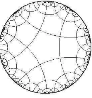
Hyperbolic graphs are a family of infinite planar graphs characterized by a cycle periodic structure. They can be briefly described as follows (for their detailed construction see, e.g., [22], or Section 2 of ref. [27]). Consider a planar graph in which each vertex has the same degree, denoted by v, and each face (ortile) is equilateral with constant number of sides denoted bys. If the parameters
Figure 2.1:The hyperbolic graphH(4, 5)in the Poincaré disc representation.
The typical representation of hyperbolic graphs make use of the Poincaré disc that is in bi-univocal correspondence withH2 (see Fig. 2.1).
Hyperbolic graphs are nonamenable, with edge isoperimetric constant explicitly computed in[11]
as a function ofvands. Moreover, the following holds:
Lemma 2.3. For all couples (v,s) such that s ≥ 4 and v ≥ 5, or s = 3 and v ≥ 9, H(v,s) is a (g,o)-growing graph for every vertex o∈V and with parameter g=g(v,s).
The proof of this Lemma is postponed to Section 5, where we will also construct a growing graph that will serve us as further example of influence of boundary conditions on the mixing time.
Let us stress, that due to the possible presence of cycles in a growing graph, a careful analysis of the correlations between spins will be required. This is actually the main distinction between our proof and the similar work on trees[26].
2.2
Ising model on nonamenable graphs
The Ising model on nonamenable graphs has been investigated in many papers (see, e.g,[20]for a survey). A general result, concerning the uniqueness/non-uniqueness phase transition of the model, is the following[15]:
Theorem 2.4(Jonasson and Steif). If G is a connected nonamenable graph with bounded degree, then there exists an inverse temperatureβ0>0, depending on the graph, such that for allβ≥β0there exists an interval of h where G exhibits a phase transition.
Thus, contrary to what happens on the Euclidian lattice, the Ising model on nonamenable graphs undergoes a phase transition also at non zero value of the external field.
results concerning the Ising model on these graphs, and stress which are the main differences from the model on classical lattices.
It has been proved (see[30; 33; 34]) that the Ising model onH(v,s) exhibits two different phase transitions appearing at inverse temperaturesβc≤βc′. The first one,βc, corresponds to the occur-rence of a uniqueness/non-uniqueness phase transition, while the second critical temperature refers to a change in the properties of the free boundary condition measureµf. Specifically, it is defined as
βc′ := inf{β≥βc : µf = (µ++µ−)/2}, (2.3)
whereµ+ andµ−denote the extremal measures obtained by imposing, respectively,(+)- and(−) -boundary condition. As is well explained in[34](see also[8]for more details), using the Fortuin-Kasteleyn representation it is possible to show that βc′ < ∞ for all hyperbolic graphs, in contrast to the behavior of the model on regular trees whereµf 6= (µ++µ−)/2 for all finiteβ ≥βc. From Definition 2.3 it turns out that for βc ≤ β < βc′, when this interval is not empty (see [34]), the measureµf is not a convex combination ofµ+andµ−. This implies the existence of a translation invariant Gibbs state different fromµ+andµ−, in contrast to what happens onZd [2].
Another interesting result concerning the Ising model on hyperbolic graphs, is due to Sinai and Series [30]. For low enough temperatures and h= 0, they proved the existence of uncountably many mutually singular Gibbs states which they conjectured to be extremal. This points out, once more, the difference between the system on hyperbolic graphs and on classical lattices, where it is known that the extremal measures are at most a countable number.
In this paper we are interested in the region of the phase diagram where the dynamics is highly sensitive to the boundary condition, namely when the temperature is low and the magnetic field is zero (phase coexistence region). Let us explain the model in detail and give the necessary definitions and notation.
LetG= (V,E)be an infinite(g,o)-growing graph with maximal degree∆. For anyr∈N, we denote by Br = (Vr,Er)⊂ G the ball with radiusr centered in o. When it does not create confusion, we identify the subgraphs of G with their vertex sets. Given a finite ball B ≡ Bm and an Ising spin configurationτ∈ΩG, letΩτB ⊂ {±1}B∪∂VB be the set of configurations that agree withτon ∂
VB. Analogously, for any subset A⊆ Vm and any η ∈ ΩτB, we denote by ΩηA ⊂ {±1}A∪∂VA the set of configurations that agree with η on ∂VA. The Ising model on Awithη-boundary condition (b.c.) and zero external field is thus specified by the Gibbs probability measureµηA, with support on ΩηA, defined as
µηA(σ) = 1
Z(β)exp(β
X
(x,y)∈E(A)
σxσy), (2.4)
where Z(β) is a normalizing constant and the sum runs over all pairs of nearest neighbors in the induced subgraph onA=A∪∂VA.
Similarly, the Ising model onAwith free boundary condition is specified by the Gibbs measureµA
supported on the set of configurationsΩA:={±1}A. This is defined as in (2.4) by replacing the sum overE(A)in a sum overE(A), namely cutting away the influence of the boundary∂VA. Notice that whenA=Vm,µ
η
Vm is simply the Gibbs measure onBwith boundary conditionτ(ηagrees withτon
∂VVm≡∂VB) andµVm is the Gibbs measure onB with free boundary condition.
that if f : ΩτB → R is a measurable function, the expectation of f w.r.t. µηA is given by µηA(f) =
P
σ∈Ωµ
η
A(σ)f(σ) and the variance of f w.r.t. µ η
A is given by Var η A = µ
η A(f
2)−µη A(f)
2. We usually think of them as functions ofη, that is µA(f)(η) =µηA(f)and VarA(f)(η) =VarηA(f). In particular
µA(f), VarA(f)∈ FAc.
In the following discussion we will be concerned with the Ising model onB with(+)-b.c. and we will use the abbreviationsΩ+,F andµinstead ofΩ+B,FBandµ+B, and thusµ(f)and Var(f)instead ofµ+B(f)and Var+B(f).
2.3
Glauber dynamics and mixing time
The Glauber dynamics on B with (+)-boundary condition is a continuous time Markov chain
(σ(t))t≥0onΩ+ with Markov generatorL given by
(Lf)(σ) = X
x∈B
cx(σ)f(σx)−f(σ), (2.5)
whereσx denotes the configuration obtained fromσby flipping the spin at the site x andcx(σ)is the jump rate fromσ toσx. We sometimes prefer the short notation∇xf(σ) = [f(σx)−f(σ)]. The jump rates are required to be of finite-range, uniformly positive, bounded, and they should satisfy the detailed balance condition w.r.t. the Gibbs measure µ. Although all our results apply to any choice of jump rates satisfying these hypothesis, for simplicity we will work with a specific choice calledheat-bath dynamics:
cx(σ) := µσx(σx) = 1
1+ωx(σ) where ωx(σ) := exp(2βσx
X
y∼x
σy). (2.6)
It is easy to check that the Glauber dynamics is ergodic and reversible w.r.t. the Gibbs measureµ, and so converges toµby the Perron-Frobenius Theorem. The key point is now to determine the rate of convergence of the dynamics.
A useful tool to approach this problem is thespectral gapof the generatorL, that can be defined as the inverse of the first nonzero eigenvalue ofL.
Remark 2.5. Notice that the generator L is a non-positive self-adjoint operator on ℓ2(Ω+,µ). Its
spectrum thus consists of discrete eigenvalues of finite multiplicity that can be arranged as 0=λ0 ≥ −λ1≥ −λ2≥. . . ,≥ −λN−1, if|Ω+|=N , withλi≥0.
An equivalent definition of spectral gap is given through the so calledPoincaré inequality for the measureµ. For a function f :Ω+7→R, define theDirichlet formof f associated toL by
D(f) := 1
2
X
x∈B
µcx[∇xf]2 = X
x∈B
µ(Varx(f)), (2.7)
where the second equality holds under our specific choice of jump rates. The spectral gapof the generator,cg ap(µ), is then defined as the inverse of the best constantc in thePoincaré inequality
or equivalently
cg ap(µ) := inf
½ D(f)
Var(f); Var(f)6=0
¾
. (2.9)
Denoting byPtthe Markov semigroup associated toL, with transition kernelPt(σ,η) =etL(σ,η), it easy to show that
Var(Ptf) ≤ e−2cg ap(µ)tVar(f). (2.10)
The last inequality shows that the spectral gap gives a measure of the exponential decay of the variance, and justifies the namerelaxation timefor the inverse of the spectral gap.
Moreover, lethσt denote the density of the distribution at timet of the process starting atσw.r.t. µ, i.e. hσt (η) = Pt(σ,η)
µ(η) . For 1≤p≤ ∞and a function f ∈ℓ
p(Ω+,µ), letkfk
pdenote the ℓpnorm of
f and define the time of convergence
τp =min
½
t>0 : sup σ
khσt −1kp≤e−1
¾
, (2.11)
that forp=1 is calledmixing time. A well known and useful result relatingτp to the spectral gap (see, e.g.,[28]), when specializing to the Glauber dynamics yields the following:
Theorem 2.6. On an n-vertex ball B⊂G with(τ)-boundary condition,
cg ap(µ)−1≤τ1≤cg ap(µ)−1×cn, (2.12)
whereµ=µτBand c is a positive constant independent of n.
We stress that a different choice of jump rates (here we considered the heat-bath dynamics) only affects the spectral gap by at most a constant factor. The bound stated in Theorem 2.6 is thus equivalent, apart for a multiplicative constant, for any choice of the Glauber dynamics.
Before presenting our main result, we recall that the Glauber dynamics for the Ising model on regular trees and hyperbolic graphs has been recently investigated by Peres et al. [17; 4]. In particular, they consider the free boundary dynamics on a finite ball B⊂G, G hyperbolic graph or regular tree, and prove that at all temperatures, the inverse spectral gap (relaxation time) scales at most polynomially in the size of B, with exponent α(β) ↑ ∞ as β → ∞. Let us stress again that under the same conditions, the dynamics on a cube of sizenin thed-dimensional lattice, relaxes in a time exponentially large in the surface arean(d−1)/d.
2.4
Main results
We are finally in position to state our main results.
Theorem 2.7. Let G be an infinite(o,g)-growing graph with maximal degree∆. Then, for allβ≫1, the Glauber dynamics on the n-vertex ball B with (+)-boundary condition and zero external field has spectral gapΩ(1).
This result, applied to hyperbolic graphs with sufficiently high degree, provides a convincing exam-ple of the influence of the boundary condition on the mixing time. Indeed, for allβ≫1, due to the fact that the free boundary measure onH(v,s)is a convex combination ofµ+ andµ− (see section 2.2), it is not hard to prove that the spectral gap for an n-vertex ball in the hyperbolic graph with free boundary condition, is decreasing withn. Most likely it will be of ordern−α(β), withα(β)↑ ∞
asβ → ∞, as in the lower bound given in[17; 4]. The presence of(+)-boundary condition thus gives rise to a jump of the spectral gap, and consequently it speeds up the dynamics.
Remarks.
(i) We recall that on Zd not much is known about the mixing time when β > βc, h= 0and the boundary condition is(+), though it has been conjectured that the it should be polynomial in n (see[9]and[5]).
(ii) A result similar to Theorem 2.7 has been obtained for the spectral gap, and thus for the mixing time, of the dynamics on a regular b-ary tree (see[26]). In particular it has been proved that while under free-boundary condition the mixing time on a tree of size n jumps from logn to nΘ(β)when passing a certain critical temperature, it remains of order logn at all temperatures and at all values of the magnetic field under (+)-boundary condition. However we stress that while trees do not have any cycle, growing graphs, and in general nonamenable graphs, can have many cycles, as well as the Euclidean lattices. The theorem above can thus be looked upon as an extension of this result to a class of graphs which in some respects are similar to Euclidean lattices.
(iii) At high enough temperatures (one phase region) the spectral gap of the dynamics on a ball B⊂G, where G is an infinite graph with bounded degree, is Ω(1) for all boundary conditions, as can be proved by path coupling techniques[32]. This suggests that the result of Theorem 2.7 should hold for all temperatures, as for the dynamics on regular trees, and not only forβ≫1. At the moment, what happens in the intermediate region of temperature, still remains an open question.
The following result provides a further example of influence of boundary conditions on the dynam-ics.
Theorem 2.8. For all finite g∈N, there exists an infinite(g,o)-growing graph G with bounded degree, such that, for allβ≫1, the Glauber dynamics on the n-vertex ball B with free boundary condition and zero external field has spectral gap Oe−θn, withθ=θ(g,β)>0.
Combining this with Theorem 2.6 and Theorem 2.7, we get a first rigorous example where the mix-ing time jumps abruptly from exponential to linear innwhile passing from one boundary condition to another.
We now proceed to sketch briefly the ideas and techniques used along the paper.
The second main step to prove Theorem 2.7, is deriving a Poincaré inequality for the Gibbs measure from the obtained notion of spatial mixing. This will be achieved by first deducing, via coupling tech-niques, a like-Poincaré inequality for the marginal Gibbs measure with support on suitable subsets, and then iterating the argument to recover the required estimate on the variance.
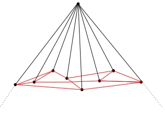
The proof of Theorem 2.8 is given by the explicit construction of a growing graph with the property of remaining "expander" even when the boundary of a finite ball is erased, as in the free measure. Using a suitable test function, we will prove the stated exponentially small upper bound on the spectral gap.
3
Mixing properties of the plus phase
In this section we analyze the effect of the(+)-boundary condition on the equilibrium properties of the system. In particular, we prove that the Gibbs measureµ≡µ+B satisfies a kind ofspatial mixing property, i.e. a form of weak dependence between spins placed at distant sites.
Before presenting the main result of this section, we need some more notation and definitions. Recall that for every integeri, we denoted byBi = (Vi,Ei)the ball of radiusicentered ino, and by
B=Bmthe ball of radiusmsuch that|Vm|=n. Let us define the following objects:
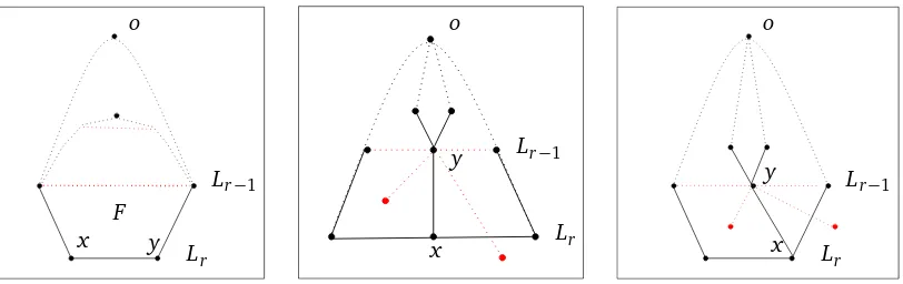
(i) thei-thlevel Li ={x∈V : d(x,o) =i} ≡∂VBi−1;
(ii) the vertex-setFi⊆Bgiven byFi := {x ∈Bci−1∩B};
(iii) theσ-algebraFi generated by the functionsπx forx∈Fic=Bi−1.
We will be mainly concerned with the Gibbs distribution on Fi with boundary condition η∈ Ω+, which we will shortly denote byµηi = µηF
i = µ(· |η∈ Fi); analogously we will denote by Var η i the variance w.r.t.µηi.
Notice that{Fi}mi=+01 is a decreasing sequence of subsets such thatVm = F0 ⊃F1⊃. . .⊃Fm+1 = ;, and in particular µi(µi+1(f)) = µi(f), for all finite i, and µm+1(f) = f. The set of variables
{µi(f)}i≥0 is a Martingale with respect to the filtration{Fi}i≥0.
For a giveni ∈ {0, . . . ,m}and a given subset S ⊂ Li, we set U = Fi+1∪S and consider the Gibbs measure conditioned on the configuration outsideU beingτ∈Ω+, which as usually will be denoted byµτU.
We are now able to state the following:
Proposition 3.1. Let G a(g,o)-growing graph with maximal degree∆. Then there exists a constant δ=δ(∆)>0such that, for everyβ > 2δ
g, everyτ∈Ω
+, and every pair of vertices x ∈S ⊂ L
i and
y∈Li\S, i∈ {0, . . . ,m},
|µτU(σx = +)−µτUy(σx = +)| ≤ce−β′d(x,y), (3.1)
withβ′:=2gβ−δ >0and for some constant c>0.
Let us briefly justify the above result. Since the boundary of B is proportional to its volume, the
prove, the effect of the(+)-boundary on a given spinσx, weakens the influence onσx coming from other spins (placed in vertices arbitrary near to x) and gives rise to the decay correlation stated in Proposition 3.1. Notice that the correlation decay increases withβ.
The proof of Proposition 3.1 is divided in two parts. First, we define a suitable event and show that the correlation between two spins is controlled by the probability of this event. Then, in the second part, we estimate this probability using a Peierls type argument. Throughout the discussion c will denote a constant which is independent of |B| = n, but may depend on the parameters ∆ and g
of the graph, and on β. The particular value of c may change from line to line as the discussion progresses.
3.1
Proof of Proposition 3.1
Let us consider two vertices x ∈S⊂ Li and y ∈ Li\S, such thatd(x,y) =ℓ, and a configuration
τ ∈ Ω+. Let τy,+ be the configuration that agrees with τ in all sites but y and has a (+)-spin on y; define analogously τy,− and denote by µUy,+ andµUy,− the measures conditioned on having respectivelyτy,+- and τy,−-b.c.. With this notation and from the obvious fact that the event {σ:
σx = +}is increasing, we get that
|µτU(σx = +)−µτUy(σx = +)| = µUy,+(σx = +)−µUy,−(σx = +). (3.2)
In the rest of the proof we will focus on the correlation in the r.h.s. of (3.2).
In order to introduce and have a better understanding of the ideas and techniques that we will use along the proof, we first consider the caseℓ=1, which is simpler but with a similar structure to the general caseℓ >1.
3.1.1 Correlation decay: the caseℓ=1
Assume thatℓ=1, namely that x and y are neighbors. Denoting byµ−U the measure with(−)-b.c. onUc=Bi\ {S}and(+)-b.c. on∂VB, we get
µUy,+(σx = +)−µUy,−(σx = +) = µUy,−(σx =−)−µUy,+(σx =−)
≤ µUy,−(σx =−)
≤ µ−U(σx =−), (3.3)
where the last inequality follows by monotonicity. The problem is thus reduced to estimate the probability of the event{σ: σx =−}w.r.t.µ−U.
LetK be the set of connected subsets ofU containing x and write
K = G
p≥1
Kp with Kp={C ∈ K s.t. |C|=p}.
For any configurationσ∈Ω+, we denote byK(σ)the maximal negative component inK admitted byσ, i.e.
K(σ)∈ K s.t.
¨
σz=− ∀z∈K(σ)
With this notation the event{σ: σx =−}can be expressed by means of disjoint events as
{σ: σx =−} = G
p≥1
G
C∈ Kp
{σ: K(σ) = C}, (3.5)
and then
µ−U(σx =−) = X
p≥1
X
C∈ Kp
µ−U(K(σ)=C). (3.6)
Let us introduce the symbolσ∼C for a configuration σsuch thatσC =−andσ∂
VC∩U = +. The main step in the proof is to show the following claim:
Claim 3.2. If G is a(g,o)-growing graph with maximal degree∆, then, for any subset C⊂U,
µ−U(σ∼C)≤e−2gβ|C|. (3.7)
The proof of Claim 3.2 is postponed to subsection 3.2. Let us assume for the moment its validity and complete the proof of the caseℓ=1. By Claim 3.2 and from the definition ofK(σ), we get
µ−U(K(σ)=C)≤e−2gβ|C|. (3.8)
We now recall the following Lemma due to Kesten (see[16]).
Lemma 3.3. Let G an infinite graph with maximum degree∆ and letCp be the set of connected sets with p vertices containing a fixed vertex v. Then|Cp| ≤(e(∆ +1))p.
Applying Lemma 3.3 to the set Kp, we obtain the bound |Kp| ≤ eδp, withδ = 1+log(∆ +1). Continuing from (3.6), we finally get that for allβ′=2gβ−δ >0, i.e. for allβ > δ
2g,
µ−U(σx =−) ≤ X
p≥1
X
C∈ Kp
e−2gβp
≤ X
p≥1
e−2gβpeδp
≤ ce−β′ (3.9)
which concludes the proof of (3.1) in the caseℓ=1.
Notice that the argument above only involves the spin atx, and thus applies for all pairs ofx,y∈Li, independently of their distance. Anyway, whend(x,y)>1 this method does not provide the decay with the distance stated in Proposition 3.1, and a different approach is required.
3.1.2 Correlation decay: the caseℓ >1
starting from y crosses a(+)-spin before arriving to x, then the communication between them is interrupted. Let us formalize this assertion.
We denote by C the set of connected subsets C ⊆ U ∪ {y}such that y ∈ C, and call an element
C ∈ C acomponentof y. For every configurationσ∈Ω+, we defineC(σ)as the maximal component of y which is negative onC(σ)∩U, i.e
C(σ)∈ C s.t.
¨
σz=− ∀z∈C(σ)∩U
σz= + ∀z∈∂VC(σ)∩U . (3.10)
Observe that the spin on y is not fixed under the event {σ: C(σ) = C}. Finally, let C; := {C ∈ C s.t. x 6∈C}and define the event
A:= {σ: C(σ)∈ C;} = G
C∈C;
{σ: C(σ)=C}. (3.11)
Then we have
µUy,−(σx = +|A) = X
C∈C;
µUy,−(σx = +,C(σ)=C|A)
=
P
C∈C;µ
y,−
U (σx = +,C(σ)=C)
P
C∈C;µy,
−
U (C(σ)=C)
=
P
C∈C;µy,
−
U (σx = +|C(σ)=C)µ y,−
U (C
(σ)=C)
P
C∈C;µ
y,−
U (C(σ)=C)
≥ min C∈C;µ
y,−
U (σx = +|C(σ)=C). (3.12)
Notice that when the measureµUy,− is conditioned on the event {σ: C(σ)= C}, the spin configu-ration on∂VC is completely determined by the boundary condition: on ∂VC∩U it is given by all
(+)-spins and on∂VC∩Ucit corresponds toτy,−. Hence, spins onU\(C∪∂
VC)become independent of spins onC, and we get
µUy,−(· |C(σ)=C) = µKy,−
x (· |σz= +,z∈∂VC∩U)
= µUy,+(· |σz= +,z∈(C∪∂VC)∩U)
≥ µUy,+(·), (3.13)
where the last inequality follows by stochastic domination. Being{σ: σx = +}an increasing event, and from (3.12) and (3.13), we get
µUy,−(σx = +|A)≥µUy,+(σx= +),
which with the obvious fact thatµUy,−(σx = +) ≥µUy,−(σx = +|A)µUy,−(A), implies
µUy,+(σx = +)−µUy,−(σx = +) ≤ µUy,−(Ac). (3.14)
LetC6=;denote the set of components of y containing x, and for every p∈N, letCp be the set of components inC6=;withpvertices, i.e
Cp:={C ∈ C6=; s.t. |C|=p} C6=;:= G
p>0
Cp.
Notice that ifC ∈ C6=;, then|C| ≥ℓ+1, since d(x,y) =ℓ. Thus,Accan be expressed by means of disjoint events as
Ac = G
p≥ℓ+1
G
C∈ Cp
{σ: C(σ) = C}, (3.15)
and we get
µ−U(Ac) = X
p≥ℓ+1
X
C∈ Cp
µ−U(C(σ)=C). (3.16)
Since ∂V(C \ {y})∩U ⊆ ∂VC ∩U, we observe that the event {σ : C(σ) = C} ≡ {σ : σC\{y} =
−,σ∂
VC∩U = +}is a subset of{σ: σC\{y}=−,σ∂V(C\{y})∩U= +} ≡ {σ:σ∼C\ {y}}. Applying the result stated in Claim 3.2 to the setC\ {y}, we obtain the bound
µ−U(C(σ)=C)≤e−2gβ(|C|−1), (3.17)
which holds under the same hypothesis of the claim. Continuing from (3.16), we then have that for allβ′=2gβ−δ >0, i.e. for allβ > δ
2g,
µ−U(Ac) ≤ X
p≥ℓ+1
X
C∈ Cp
e−2gβ(p−1)
≤ eδX
p≥ℓ
e−(2gβ−δ)p
≤ ce−β′ℓ, (3.18)
where in the second line we used the bound|Cp| ≤eδpdue to Lemma 3.3. This concludes the proof of Proposition 3.1. In the next subsection we will go back and prove Claim 3.2.
3.2
Proof of Claim 3.2
To estimate the probabilityµ−U(σ∼ C), we now appeal to a kind of Peierls argument that runs as follows (see also[15]). Given a subsetC ⊆U, we consider the edge boundary∂EC and define
∂+C := {e= (z,w)∈∂EC : z,w∈U}
∂−C := {e= (z,w)∈∂EC : zor w∈Uc} . (3.19)
The meaning of this notation can be better understood if we consider a configurationσ∈Ω−U such that C(σ)= C (see (3.10)). In this caseσhas(−)-spins on both the end-vertices of every edge in
∂−C and a (+)-spin in one end-vertex of every edge in∂+C. Similarly if we considerσsuch that
K(σ)=C (see (3.4)).
Hamiltonian contribute of the interactions just along the edges in∂EC. In particular σ∗ loses the positive contribute of the edges in∂+C and gains the contribute of the edges in∂−C, and then we get
HU−(σ∗) = H−U(σ)−2(|∂+C| − |∂−C|). (3.20)
From this, we have
µ−U(σ∼C) = X
{σ:σ∼C}
e−βH−U(σ)
ZU−
≤
P
{σ:σ∼C}e−βH
−
U(σ)
P
{σ:σ∼C}e−βH
−
U(σ∗)
= e−2β(|∂+C|−|∂−C|), (3.21)
where in the first inequality we reduced the partition function to a summation over{σ:σ∼C}and then we applied (3.20).
The following Lemma concludes the proof of Claim 3.2.
Lemma 3.4. Let G a(g,o)-growing graph with maximal degree∆. Then, for every subset C⊆U,
|∂+C| − |∂−C| ≥ g|C|. (3.22)
Proof. For a subsetC ⊆U, we define the downward boundary of C,∂↓C, as the edges of∂EC such that the endpoint inC is in a higher level (strictly small index) than the endpoint not inC, i.e.
∂↓C ={(u,v)∈∂EC:∃js.t. u∈Lj∩C, v∈Lj+1}.
We then define the not-downward boundary ofC,∂C, as the edges in∂EC which are not-downward edges, i.e. ∂C =∂EC\∂↓C.
Notice that∂↓C⊆∂+C, while∂C⊇∂−C. In particular, inequality (3.22) follows from the bound
|∂↓C| − |∂C| ≥g|C|. (3.23)
For all j≥0, defineCj=C∩Lj and notice that, by the growing property ofG,
|∂↓Cj| − |∂Cj| ≥g|Cj|. (3.24)
Moreover, one can easily realize that
|∂↓C| − |∂C|=X
j≥0
|∂↓Cj| − |∂Cj|. (3.25)
4
Fast mixing inside the plus phase
In this section we will prove that the spectral gap of the Glauber dynamics, in the situation described by Theorem 2.7, is bounded from zero uniformly in the size of the system. From Definition 2.9 of spectral gap, this is equivalent to showing that for all inverse temperature β ≫ 1, the Poincaré inequality
Var(f)≤cD(f), ∀f ∈L2(Ω+,F,µ)
holds with constantcindependent of the size ofB.
First, we give a brief sketch of the proof. The rest of the section is divided into two parts. In the first part, from the mixing property deduced in section 3 and by means of coupling techniques, we derive a Poincaré inequality for some suitable marginal Gibbs measures. Then, in the second part, we will run a recursive argument that together with some estimates, also derived from Proposition 3.1, will yield the Poincaré inequality for the global Gibbs measureµ.
4.1
Plan of the Proof
Let us first recall the following decomposition property of the variance which holds for all subsets
D⊆C⊆B,
VarηC(f) = µηC[VarD(f)] +Var η
C[µD(f)]. (4.1)
Applying recursively (4.1) to subsets B ≡ F0 ⊃ F1 ⊃ . . . ⊃ Fm+1 = ; and recalling the relations
µi(µi+1(f)) = µi(f)andµm+1(f) = f, we obtain
Var(f) = µ[Varm(f)] +Var[µm(f)]
= µ[Varm(µm+1(f))] +µ[Varm−1(µm(f))] +Var[µm−1(µm(f))]
= ...
=
m
X
i=0
µ[Vari(µi+1(f))]. (4.2)
Notice that (4.2) can also be seen as a decomposition of the Martingale given by the set of variables
{µi(f)}i≥0 respect to the filtration{Fi}i≥0.
To simplify the notation we definegi := µi(f)for alli=0, . . . ,m+1. Notice thatgi∈ Fi. Inserting
gi in (4.2), we then have that
Var(f) =
m
X
i=0
µ[Vari(gi+1)]. (4.3)
The proof of the Poincaré inequality forµ, with constant independent of the size of the system, is given in the following two steps:
1. Proving that∀τ∈Ω+andi∈ {0, . . . ,m}, there exist suitable vertex-subsets{Kx}x∈Li,Kx∋x, such that the like-Poincaré inequality
Varτi(gi+1)≤c X
x∈Li
µτi(VarK
x(gi+1)) (4.4)
2. Relating the variance of gi = µi(f) to the variance of f in order to get an inequality of the kind
m
X
i=0
X
x∈Li
µ(VarK
x(gi+1))≤cD(f) +ǫ m
X
i=0
X
x∈Li
µ(VarK
x(gi+1)) (4.5)
withǫa small quantity forβ≫1.
Notice that from (4.5) the inequality
m
X
i=0
X
x∈Li
µ(VarK
x(gi+1))≤c(1−ǫ)
−1D(f)
follows withc(1−ǫ)−1= Ω(1)for allβ≫1. Together with Eqs. (4.3) and (4.4), this will establish the required Poincaré inequality forµand therefore will conclude the proof of Theorem 2.7.
4.2
Step 1: From correlation decay to Poincaré inequality
In this section we prove that under the same hypothesis of Proposition 3.1, the marginal of the conditioned Gibbs measure on some suitable subsets, satisfies a Poincaré inequality with constant independent of the size of these subsets.
To state the result, let us fix a subsetS⊆ Li and a configurationτ∈Ω+. We then define the measure
νSτ(σ) := X
η:ηS=σS
µ(η|τ∈ FBi\S), (4.6)
which is the marginal of the Gibbs measureµτF
i+1∪S onS, and denote by Varν
τ
S the variance w.r.t.ν τ S. We state the following:
Theorem 4.1. For allβ≫1and for every subset S⊆Li,τ∈Ω+and f ∈L2(Ω,FS,νSτ), the measure νSτsatisfies the Poincaré inequality
Varντ
S(f)≤c0
X
x∈S
νSτ(Varx(f)). (4.7)
with c0=c0(β,∆,g) =1+O(e−cβ).
Remark 4.2. Before proceeding with the proof of Theorem 4.1, we point out that this result includes, as a particular case, inequality (4.4) for subsets Kx = Fi+1∪ {x}. To see that, choose S = Li so that
µ(· |FB
i\S)≡µi. An easy computation shows that, for every function f ∈ Fi+1,ν τ
Li(f)≡µ τ
i(f)and
νLτ
i(Varx(f)) =µ τ
i(VarKx(f)). Inequality (4.7) then corresponds to the like-Poincaré inequality
Varτi(gi+1)≤c0
X
x∈Li
µτi(VarKx(gi+1)),
4.2.1 Proof of Theorem 4.1
The proof of Theorem 4.1 rests on the so called coupling technique. This is a useful method to bound from above the mixing time of Markov processes, introduced for the first time in this setting by Aldous [1] and subsequently refined to the path coupling [3; 21]. See also [18] for a wider discussion on the coupling method.
Acouplingof two measureµ1andµ2onΩis any joint distributionρonΩ×Ωwhose marginal are
µ1 andµ2 respectively. Here, we want to construct a coupling of two Glauber dynamics onΩS with same reversible measureνSτ but different initial configurations. We denote by LS the generator of this dynamics. We also recall that for allη∈ΩτS, x ∈S anda ∈ {±1}, the jump rates of the heat bath version of the dynamics (see Def. 2.6 ) are given by
cx(η,a) = νSτ(σx =a|η∈ FS\x)
= µ(σx =a|η∈ FS\x,τ∈ FB
i\S)
= µηK
x(σx =a), (4.8)
where in the second line we applied the definition ofνSτ and used that{σx = a} ∈ FS, and in the last line we adopt the notationKx :=Fi+1∪ {x}.
We now consider the coupled process(η(t),ξ(t))t≥0onΩS×ΩSdefined as follows. Given the initial configurations(η,ξ), we let the two dynamics evolve at the same time and update the configurations at the same vertex. We then chose the coupling jump rates ˜cx((η,a),(ξ,b)) to go from (η,ξ) to
(ηx,a,ξx,b), witha,b∈ {±1}, as the optimal coupling (see[18]) between the jump ratesµη Kx(σx =
a)andµξK
x(σx =b). More explicitly, fora∈ {±1}, they are given by
(
˜
cx((η,a),(ξ,a)) =min{µηK
x(σx =a);µ ξ
Kx(σx =a)} ˜
cx((η,a),(ξ,−a)) =max{0 ;µ η
Kx(σx =a)−µ ξ
Kx(σx=a)}
(4.9)
We denote byLfthe generator of the coupled process, and by ePt the correspondent Markov semi-group. Notice that from our choice of coupling jump rates, we get that the probability of disagree-ment inx, after one update inx of(η,ξ), is given by
Pd isx (η,ξ):=|µηK
x(σx = +)−µ ξ
Kx(σx = +)|. (4.10)
Let us now consider the subsetH ⊂ΩS×ΩS given by all couples of configurations which differ by a single spin flip in some vertex ofS. One can easily verify that the graph(ΩS,H)is connected and that the induced graph distance between configurations(η,ξ)∈ΩS×ΩS, D(η,ξ), just corresponds to their Hamming distance. Let us also denote byEη,ξ[D(η(t),ξ(t))]the average distance at timet
between two coupled configurations of the process starting at(η,ξ). We claim the following:
Claim 4.3. For allβ ≫1, there exists a positive constant α≡α(β,g,∆) such that, for every initial configurations(η,ξ)∈H, the process(η(t),ξ(t))t≥0satisfies the inequality
d
d tEη,ξ[D(η(t),ξ(t))]
¯
Proof of Claim 4.3. The derivative in t of the average distance, computed for t =0, can be written as
d
d tEη,ξ[D(η(t),ξ(t))]
¯
¯t=0 = d d t
e
PtD(η,ξ)¯¯t=0 = (LfD)(η,ξ)
=X
x∈S
X
a,b∈{±1}
˜
cx((η,a)(ξ,b))[D(ηx,a,ξx,b)−D(η,ξ)]. (4.12)
Since(η,ξ)∈H, there exists a vertex y ∈S such that ξ=ηy. If x = y, then Px d is(η,η
x) =0 and
the distance between the updated configurations decreases of one. While ifx 6= y, with probability
Pd isx (η,ηy)the updated configurations have different spin at x and their distance increases by one. Continuing from (4.12) we get, for allβ≫1,
d
d tEη,ξ[D(η(t),ξ(t))]
¯
¯t=0 = −1+X
x∈S x6=y
Pd isx (η,ηy)
≤ −1+cX
ℓ≥1
e−β′ℓ∆ℓ
≤ −(1−ce−β′), (4.13)
where in the second line we used the bound
Pd isx (η,ηy) =|µηK
x(σx = +)−µ ηy
Kx(σx = +)| ≤ce
−β′d(x,y), (4.14)
which holds for all β′ =δβ−2g >0 as stated in Proposition 3.1. Claim 4.3 follows taking α = (1−ce−β′)andβ sufficiently large.
Using thepath couplingtechnique (see[3]) we can extend the result of Claim 4.3 to arbitrary initial configurations(η,ξ)∈ΩS×ΩS, and obtain
d
d tEη,ξ[D(η(t),ξ(t))]
¯
¯t=0 ≤ −αD(η,ξ). (4.15)
From (4.15) it now follows straightforwardly thatEη,ξ[D(η(t),ξ(t))]≤e−αtD(η,ξ), and then we get
P(η(t)6=ξ(t))≤Eη,ξ(D(η(t),ξ(t)))≤e−αtD(η,ξ). (4.16)
To bound the spectral gap cg ap(νSτ) of the dynamics on S, we consider an eigenfunction f ofLS with eigenvalue−cg ap(νSτ), so that
Eσf(η(t)) =etLSf(η) = e−cg ap(νSτ)tf(η).
Since the identity function has eigenvalue zero, and therefore it is orthogonal to f, it follows that
νSτ(f) =0 andνSτ(Eξf(ξ(t))) =0, whereνSτ is the invariant measure forLS. From these consider-ations and inequality (4.16), we have
etLSf(σ) = E
ηf(η(t))−νSτ(Eξf(ξ(t)))
= X
ξ
νSτ(ξ)[Eηf(η(t))−Eξf(ξ(t)) ]
≤ 2kfk∞sup η,ξ
P(η(t)6=ξ(t))
From the last computation, which holds for allη∈ΩτS and for allt, we finally obtain thatcg ap(νSτ)≥ α independently of the size of S, which implies the Poincaré inequality (4.7) with constant c0 =
α−1=1+O(e−cβ). This concludes the proof of Theorem 4.1.
4.3
Step 2: Poincaré inequality for the global Gibbs measure
With the previous analysis we obtained a like-Poincaré inequality for the marginal of the measure
µi on the level Li (see Remark 4.2), which inserted in formula (4.3) provides the bound
Var(f) ≤ c0 m
X
i=0
X
x∈Li
µµi(VarK
x(gi+1))
. (4.18)
Using the same notation as in[26], let us denote the sum in the r.h.s. of (4.18) by Pvar(f). The aim of the following analysis is to study Pvar(f)in order to find an inequality of the kind Pvar(f)≤ cD(f) +ǫPvar(f), withǫ=ǫ(β,g,∆)<1 independent of the size of the system. This would imply that
Var(f)≤c0·Pvar(f)≤c0 c
1−ǫD(f),
and then would conclude the proof of Theorem 2.7.
In this last part of the section, we will first relate the local variance of gi = µi(f) with the local variance of f. This will produce a covariance term that will be analyzed using a recursive argument.
4.3.1 Reduction to covariance
In order to reconstruct the Dirichlet form of f from (4.18), we want to extract the local variance of
f from the local variance of gi+1. Notice that w.r.t. the measureµKx, the function gi+1just depends on x. Fixing x ∈Li andτ∈Ω+, and definingp(τ):=µτK
x(σx = +)andq(τ):=µ τ
Kx(σx =−), we can write
µiVarK x(gi+1)
= X
τ
µi(τ)p(τ)q(τ) (∇x gi+1(τ))2. (4.19)
Using the martingale propertygi+1=µi+1(gi+2), the variance VarKx(gi+1)can be split in two terms, stressing the dependence on x ofgi+2 and of the conditioned measureµi+1. Let us formalize this idea.
For a given configurationτ∈Ω+we introduce the symbols
τ+ :=
¨
τ+y =τy if y 6=x
τ+y = + if y =x τ
− :=
¨
τ−y =τy if y6=x τ−y =− if y =x
and define the density
hx(σ):= µ
τ+
i+1(σ)
µτi+−1(σ), with µ
τ−
Whit this notation and continuing from (4.19), we get
with the fact that ∇xf does not depend on x, means that the expression on the r.h.s. of (4.22) equals to
where we denoted byµ−i+1 the measure conditioned on having all minus spins inBi and plus spins in∂VB. Inequality (3.9), applied toU =Fi+1, implies that
withβ′=2gβ−δas in Proposition 3.1. Combining (4.26) and (4.27), we get that for allβ≥2δ
g,
khxk∞≤1+ce−β′. (4.28)
Altogether, inequalities (4.22)-(4.28) imply that
X
τ
µi(τ)p(τ)q(τ)
µτi++1(∇xgi+2)
2
≤c1µi Varx(f), (4.29)
with c1 = c1(β,∆,g) = 1+O(e−cβ). Thus, summing both sides of (4.21) over x ∈ Li and i ∈ {0, . . . ,m}, and applying inequality (4.29), we obtain
Pvar(f) ≤ 2c1D(f) +2 m
X
i=0
X
x∈Li
µ
X
τ
µi(τ)p(τ)q(τ)µτi+−1(hx,gi+2)
2
. (4.30)
Notice that sincegm+2≡ f is constant w.r.t. µm+1, thenµτ
−
m+1(hx,gm+2)≡0 and the valuemcan be removed from the summation overiin the r.h.s. of (4.30).
It now remains to analyze the covarianceµτi+−1(hx,gi+2).
4.3.2 Recursive argument
Before going on with the proof, we need some more definitions and notation. For every x ∈Li, let
Dx denote the set of nearest neighbors of x in the levelLi+1 (descendants ofx). Given x ∈Li and
ℓ∈N, let us define the following objects:
(i) Dx,ℓ:={y∈Li+1 : d(y,Dx)≤ℓ} is theℓ-neighborhood ofDx in Li+1;
(ii) Fx,ℓ := σ
σy : y ∈Bi+1\Dx,ℓ
is theσ-algebra generated by the spins onBi+1\Dx,ℓ;
(iii) µx,ℓ(·):=µ(· |Fx,ℓ) is the Gibbs measure conditioned on theσ-algebraFx,ℓ.
We remark thatDx,0=Dx, and that there exists someℓ0≤2(i+1)such that, for all integersℓ≥ℓ0,
Dx,ℓ=Li+1 andµx,ℓ=µi+1.
We also remark that for any function f ∈ L1(Ω,Fi+1,µ), the set of variables {µx,ℓ(f)}ℓ∈N is a Martingale with respect to the filtration{Fx,ℓ}ℓ=0,1,...,ℓ
0.
Let us now come back to our proof and recall the following property of the covariance. For all subsetsD⊆C ⊆B,
µηC(f,g) = µηC(µD(f,g)) +µηC(µD(f),µD(g)). (4.31)
Since the support ofµi+1 strictly contains the support ofµx,0, we can apply the property (4.31) to the square covariance(µτi+−1(hx,gi+2))2appearing in (4.30), in order to get
(µτi+−1(hx,gi+2))2 ≤ 2(µτi+−1(µx,0(hx,gi+2)))2+2(µτi+−1(µx,0(hx),µx,0(gi+2)))2. (4.32)
The first term in the r.h.s. of (4.32) can be bounded, by the Schwartz inequality, as
(µτi+−1(µx,0(hx,gi+2)))2≤µτ
−
i+1(Varx,0(hx))·µτ
−