POLARIZED CATEGORY THEORY, MODULES,
AND GAME SEMANTICS
J.R.B. COCKETT AND R.A.G. SEELY
Abstract. Motivated by an analysis of Abramsky-Jagadeesan games, the paper con-siders a categorical semantics for a polarized notion of two-player games, a semantics which has close connections with the logic of (finite cartesian) sums and products, as well as with the multiplicative structure of linear logic. In each case, the structure is polarized, in the sense that it will be modelled by two categories, one for each of two polarities, with a module structure connecting them. These are studied in considerable detail, and a comparison is made with a different notion of polarization due to Olivier Laurent: there is an adjoint connection between the two notions.
Contents
1 Basic polarized games 8
2 Basic polarized game logic 12
3 Polarized categories 16
4 The logic of polarized cut and its semantics 24
5 Additive types for polarized polycategories 37
6 Linear polarized categories 55
7 Multiplicative and additive structure on AJ games 80
8 Depolarization 84
9 Exponential structure 88
10 Laurent polarized games 93
11 Concluding remarks 99
Introduction
The idea of developing an algebraic and proof theoretic approach to game theory has a certain level of irony, since games, viewed as combinatorial structures, are regarded as being endowed with sufficient worldliness that they pass muster as a respectable seman-tics. The temptation to reinvent them as a type theory and thereby turn this notion of semantics on its head was irresistible.
Research partially supported by NSERC, Canada. Diagrams in this paper were produced with the help of theXY-picmacros of K. Rose and R. Moore, thediagxymacros of M. Barr, andTEXCADby G. de Montmollin.
Received by the editors 2004-10-19 and, in revised form, 2007-01-18. Transmitted by Martin Hyland. Published on 2007-01-22.
2000 Mathematics Subject Classification: 18D10,18C50,03F52,68Q55,91A05,94A05.
Key words and phrases: polarized categories, polarized linear logic, game semantics, theory of com-munication.
c
J.R.B. Cockett and R.A.G. Seely, 2007. Permission to copy for private use granted.
The realization that the logic of (polarized) games is a just a subtle modification of the logic of products and sums [CS00] suggested to us that there was a rather dif-ferent approach to understanding these games. Considering the logical complexities of the commuting conversions of the logic of products and coproducts, ΣΠ [CS00], and the connections of that system with games, it is not unnatural to ask if one can avoid the conversions by introducing some extra type constraints on the type theory, and if the resulting system has a game-theoretic interpretation. The answer is in fact more far-reaching even than the example of ΣΠ might lead one to expect. The key lay in providing a categorical semantics for these subtly changed sums and products. This meant that we had to understand the categorical meaning of polarization and the related notion of “focus”.
Of course, once one puts the question in these terms, the answer inevitably is staring one in the face. The logic of a two player game cries out to be interpreted as a module between two categories. The problem then is to transport standard categorical notions into this “polarized” world. Central to this was the idea of an “inner adjoint” which has the universal properties of an adjoint but in a polarized sense.
It remained however to find a voice for this way of telling the story of polarized games amidst the altogether more practical uses of game theory and a community very focused (and rightly so) on applications of games. This paper has had a long period of gestation, and many of the ideas underlying the story we wished to tell were just beneath the surface in the community anyway, so it was not surprising that as we began to talk openly about our perspective on these games [C00, C02a, C02b], Olivier Laurent published his work on “polarized linear logic” [L02]1.
Laurent’s view of polarization, while being very similar to ours, at the same time was also subtly different. His view of polarization was heavily influenced by Girard’s view of and grouping of the connectives of linear logic. Consequently his work struck a familiar cord with many linear logicians. Furthermore, Laurent used a Hyland-Ong style game theoretic models to provide a semantics.
Inevitably, our view of the polarization of the connectives was rather different. We had taken as our starting point the games used by Abramsky and Jagadeesan [AJ92] and this had lead us to a rather different organization of the same basic material. At the end of the paper we explain the relationship between the two approaches. The main difference is two-fold: we emphasise different operators, and we include operators not included in Laurent’s presentation. Almost all these operators may be seen in the simple finitary game model that serves as our motivation in the first section. This perspective makes some important aspects of these game models explicit, which were implicit in previous treatments, such as focalization and the subtly different notions of sums and products possible in the polarized setting. The latter can be interpreted as different communication strategies which we discuss in sections 4, 5.
For example, we describe a “depolarization” process which can take a polarized model and produce a∗-autonomous category,i.e. a non-polarized model of (multiplicative) linear logic. The navigation of the polarized additive connectives and their role in depolarization
1Laurent has published several variants of his polarized logic; for definiteness our comments refer to
is sufficiently complex that, without a careful treatment of these connectives, it is not easy to see what properties are required of the polarized model to ensure the depolarization has multiplicatives. The choices made, for example, by Laurent do not support depolarization with multiplicatives. On the other hand, the choices implicit in Abramsky and Jagadeesan are precisely sufficient to provide a depolarization with multiplicatives. However, they are not sufficient to deliver additives, which requires a different additive structure, as we shall discuss in section 8.2.
Furthermore, we note that our notion of polarization is compatible with the co-Kleisli construction in the presence of the “exponentials” ! and ? — in fact, given a polarized game category with a suitable notion of ! and ?, there is a polarized co-Kleisli construc-tion which lifts the semantics to include these exponentials. Such a construcconstruc-tion doesn’t “type” in the Laurent setting, and cannot work in such a simple fashion.
Lest anyone think otherwise, we should make clear that we do not take the view that one approach is superior to the other. There may be many notions of polarization, each with its own virtues and special properties, and we hope adherence to one will not preclude readers from the delights of others. Laurent polarization provides a series of categorical doctrines which are parallel to ours. In fact, they are linked to our doctrines by adjunctions which use the family construction to freely add non-polarized additives.
The publication of Laurent’s work did cause us to wonder again whether there was sufficient left in the story we wished to tell. Laurent’s work had, for example, provided a very compact (one sided) sequent presentation for games. We had felt that our sequent presentation was a highlight — indeed a novelty — of our work. But although we can no longer claim originality for providing a sequent logic for these polarized games, we do claim our systems have some interesting features. One dubious distinction is that our systems have many more rules! However there are some good reasons for this. We take a very basic approach to these logics, making sure that they correspond transparently to their categorical semantics. However, this is not the real source of their size; rather, it is our continued insistence that these systems need have neither negation nor a commutative multiplicative structure. Thus the calculi we consider are more general those presented in Laurent’s work; but more important is that ours are very modular (features are added only as needed). We think that the real gain is in the explicit nature of the resulting logic. The story of this game theory has been told many times, often with the intent of getting the reader to the applications in the semantics of programming as fast as possible [H97, A97]. In this context it has become usual to regard games as being combinatorial structures and thus to be imbued with sufficient concreteness to be passable as a semantics. This is not the story we wish to tell here: we take (in common with Laurent) a very proof theoretic approach and when we talk of semantics we are thinking of the categorical models of the proof theory which have as little claim to concreteness as the proof theory itself. To be sure, we regard it as remarkable and fortuitous that the initial models have a concrete combinatorial description. However, our primary interest in them stems from the fact that they are the result of general constructions and that these constructions allow movement, at a general level, from one categorical doctrine to another.
regard as a starting point for understanding the categorical semantics of polarized games, is also original to our particular way of telling the story.
Part I
The basic game situation
1. Basic polarized games
To begin with we shall present a type system which we claim accounts for the basic structure of 2–player input–output games, of the sort studied (in the context of semantics of linear logic) by Abramsky and Jagadeesan [A97]. We consider this as an example of a general process; we shall probe this special case as an illustration, but do not regard it as exhausting the techniques or ideas behind this paper. For example, although we do not consider Conway games in this paper, these appear to be susceptible to a similar treatment albeit with rather different type theory.2 We shall start with a simple type theory for games; however it is not sufficient to handle game constructors such as tensor and par. In later sections we shall show how those may be handled by a richer system, which may be more easily understood after the simpler system has been presented. In addition, we shall present a categorical semantics for these type theories in terms of polarized sums and products.
The games we wish to abstract have two players: Othe “opponent” andPthe “player”, each of which has associated moves. When the morphisms between these games are viewed as processes, it is natural to think of the moves as messages which are being passed between processes. It is then usual to classify these messages from a “system centric” perspective: those which originate from the environment and those which are generated by the process or system itself. In the codomain of a morphism it is possible to identify the system messages with player moves and environment messages with the opponent moves. However, in the domain these roles are completely reversed: system message are identified with opponent moves and environment messages with player moves. An important characteristic of a game is whether the opponent or player starts, as this determines the direction of the initial message.
Since initially we shall not consider type constructors like “internal hom” we cannot follow the more usual approach of coding a morphism up as a strategy for a single game (of typeA−◦B). Instead we have to explicitly define the morphisms between our games. To facilitate this, in the next section we shall think of games as types and morphisms between games as proofs, derivations, or terms, in a manner familiar from type theory. The fact that there are opponent and player games necessitates that the type theory has opponent and player sequents which accommodate the different sorts of games which are available. In addition our basic type theory will have two constructions which allow us to build games as trees whose paths consist of alternating sequences ofO-moves andP-moves. Given any finite family {Xi}i∈I of O-games, we can construct a P-game Fi∈IXi and dually given any finite family {Yj}j∈J of P-games, we can construct an O-game dj∈JYj. To allow a connection betweenO-sequents andP-sequents we shall need “mixed” or “cross” sequents which operate between O-games and P-games.
To illustrate the structure we have in mind, we shall start with a variant3 of a
well-2
At times we shall refer to “combinatorial games”; in this paper, by that phrase we shall mean Abramsky-Jagadeesan style games, not Conway games.
“Abramsky-known model, viz. Abramsky-Jagadeesan games [A97] which actually gives the initial categorical model of the basic type theory we shall introduce. We start by explaining this model from the present point of view to motivate the abstractions we shall make with our type theories. In case the reader gets the wrong impression, however, we should remark here that the infinitary games, with strategies (and winning strategies), may be presented as a model of the following framework as well, although we think the finitary variant gives a clearer model, and has the additional virtue of being a free model of the basic logic. The syntax we present below has no explicit reference to strategies, however. The appropriate level of categorical generalization of strategies is still unclear to us, and will have to await a sequel. An idea of a possible approach may be found in the “glueing” example, 3.0.2.
1.1. Polarized (finite) AJ games.Here a game may be regarded as a finite labeled bipartite tree: the nodes are partitioned into player states and opponent states and a labeled edge is required to start in a different partition from where it ends. When the root is a player node we shall call the game a player game and similarly if the root is an opponent node we shall call it a opponent game.
We shall use several notations for these games. • A player game is denoted
P ={ai:Oi |i∈I}=G i∈I
ai:Oi
where each Oi is an opponent game. Moreover, supposing I = {1,2, . . . , n}, we could represent this by the following graph.
✉ ☎ ☎ ☎
❜ ❜
❜ ❜❜
a1a2 an
O1 O2 On
. . .
• An opponent game is denoted
O = (bj:Pj |j ∈J) =
l
j∈J bj:Pj
where each Pj is a player game. Again, this might be represented as this graph.
❡ ☎ ☎ ☎
❜ ❜
❜ ❜❜
b1 b2 bn
P1 P2 Pn
. . .
The binary versions of the basic operations are O⊔O′, which takes two opponent games
and produces a player game, and P ⊓P′, which takes two player games and produces an
opponent game. The atomic games are given when the index sets are empty. We shall denote these by 0=F∅ ={ } and 1=d∅ = ( ). Graphically, these are just leaves on a tree.
Given a game G there is a dual game G which is obtained by swapping products for sums and overlining the component indicators (where we assume that double overlining is the identity). Thus, we have:
P = Fi∈Iai:Oi = di∈Iai:Oi = (ai:Oi |i∈I) Q = dj∈Jbj:Pj = Fj∈Jbj:Pj = {bj:Pj |j ∈J}
Our basic game type theory will abstract just this basic F−d structure, but these games carry some additional structure which we will present in a later section, and which motivates the multiplicative extension of the basic type theory.
1.2. Maps and strategies.The usual way to specify maps between these games isvia
strategies and counter-strategies. However we shall adopt a somewhat different approach by directly describing the morphisms between games. Strategies can then be recovered as morphisms from the final game 1 (and counter-strategies as morphisms to the initial game 0): using the closed structure which we introduce later we can recover the usual definition of the morphisms (see Proposition 7.2.2).
[Opponent maps:]
b1 7→ h1 · · · bm 7→ hm
:O //(b1:P1, . . . , bm:Pm)
where each hi:O //Pi is a mixed map. We shall occasionally use the in-line notation (bi:hi)i∈I:O //(bi:Pi |i∈ I). Note that the displayed notation has the advantage of not needing subscripts, since the tokens may play that role themselves. [Mixed maps:] These are either of the form
−
→ak·g:O //{a1:O1, . . . , an:On}
where k∈ {1, . . . , n}, and g:O //Ok is an opponent map, or ←−
bk ·f: (b1:P1, . . . , bn:Pn) //P
where k ∈ {1, . . . , n}, and f:Pk //P is a player map. When the subscript is not necessary (being specified by the token itself) we may drop it.
[Player maps:]
a1 7→ h1 · · · am 7→ hm
:{a1:O1, . . . , am:Om} //P
1.2.1. Remark.Note that this notation gives in effect a notational comparison between CCS and theπ-calculus on one side, and the categorical notions of product and coproduct on the other. This is intended, and reflects a basic intuition behind this work. This is made even more explicit in the thesis of Craig Pastro [P03].
1.2.2. Example. Here is a map between two opponent games:
Here are four mixed maps between these given games:
1. ←−a ·
1.3.1. Example. Here is a reduction of an opponent map composed with a mixed map.
It is an easy inductive argument to show that this is a confluent and terminating rewriting which eliminates the composition (as we shall shortly see this is a cut-elimination procedure). Furthermore, these rewritings satisfy the associative law in all the configu-rations which are possible. (See [CS00] for proofs for a similar system — in fact those proofs carry over to the present context, and even become simpler since the permuting conversions of [CS00] are absent in the present context.)
1.3.2. Lemma.
(i) The above rewriting on maps terminates.
(ii) The above rewriting on maps is confluent.
(iii) The associative law is satisfied by all composible triples.
To establish categorical structure for games and morphisms, we must exhibit the appropriate identity maps.
Given a player objectP ={ai:Oi |i∈I}we define the identity map 1P ={−→ai·1Oi}i∈I;
given O = (bi:Pi |i∈I) we define its identity map 1O = (←bi−·1Pi)i∈I. We then have: 1.3.3. Lemma.In any possible composition with an identity, the identity acts as a neutral element with respect to that composition.
As will be seen in section 3, this means that we have two categories, the player and the opponent category, linked by a module (see Definition 3.0.1). In that section we give a complete characterization of the categorical models which in addition to being a module must possess polarized products and sums.
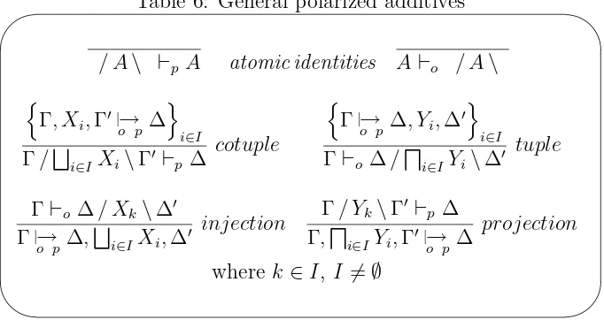
2. Basic polarized game logic
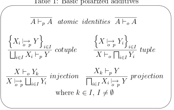
Table 1: Basic polarized additives
✬
✫
✩
✪
A⊢p A atomic identities A⊢o A
n
Xi o→ p Y
o
i∈I
F
i∈IXi ⊢p Y
cotuple
n
X o→ p Yi
o
i∈I X ⊢o di∈IYi
tuple
X ⊢o Yk X o→
p
F
i∈IYi
injection dXk ⊢p Y
i∈IXi o→p Y
projection
where k ∈I, I 6=∅
structure, together with a cut elimination process, which will motivate and justify the categorical structure presented later. This basic game logic will be a bit peculiar since we shall need three kinds of sequents:
Player sequents: These take the form:
X ⊢p Y
where X and Y are player propositions.
Opponent sequents: These are dual to the player sequents, they take the form: V ⊢o W
where V and W are opponent propositions.
Cross sequents: These are self-dual and have the form: V o→
p Y
where V is an opponent proposition andY is a player proposition.
The valid inferences are generated from the rules in Table 1, which are a “graded” version of ΣΠ [CS00].
Notice that the rules are symmetric: the symmetry is given by swapping the direction of the sequents while at the same time swapping “player” for “opponent” and F for d. This symmetry arises from an underlying categorical duality.
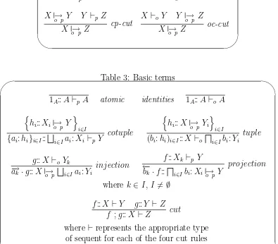
Table 2: Basic cut rules
✬
✫
✩
✪
X ⊢p Y Y ⊢p Z X ⊢p Z
p-cut X ⊢o Y Y ⊢oZ
X ⊢o Z o-cut
X o→
p Y Y ⊢p Z X o→
p Z
cp-cut X ⊢o Y Y o→p Z
X o→ p Z
oc-cut
Table 3: Basic terms
✬
✫
✩
✪
1A::A⊢p A atomic identities 1A::A⊢o A
n
hi::Xi o→ p Y
o
i∈I {ai:hi}i∈I::Fi∈Iai:Xi ⊢p Y
cotuple
n
hi::X o→ p Yi
o
i∈I (bi:hi)i∈I::X ⊢odi∈Ibi:Yi
tuple
g::X ⊢o Yk −
→ak·g::X o→p
F
i∈Iai:Yi
injection ←− f::Xk ⊢p Y bk ·f::di∈Ibi:Xi o→
p Y
projection
where k ∈I, I 6=∅ f::X ⊢Y g::Y ⊢Z
f ;g::X ⊢Z cut
where ⊢represents the appropriate type of sequent for each of the four cut rules
2.1. A term logic. In fact more is true. As for ΣΠ we may assign terms to this logic (Tables 3 and 4): however, where ΣΠ needed commuting conversions this logic does not because the type system makes the conversions impossible. Essentially this means that it is possible to have combinatorial models for these game processes as there are no manipulations once cut has been eliminated. The terms and term rewrites are similar to the ones we listed for polarized AJ games. To reduce the overload strain on colons, we use :: to denote the term-type membership relation, sot::U ⊢V will mean thatt is a term of type U ⊢ V, where U (say) may be of the form a:X. Then we can assert that cut elimination steps preserve the equivalence on terms induced by these rewrites.
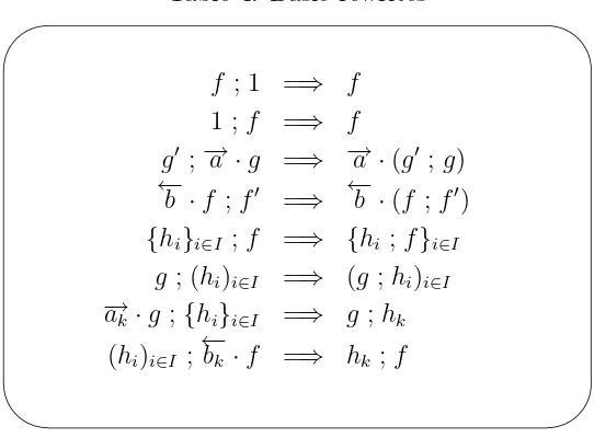
Table 4: Basic rewrites
✬
✫
✩
✪
f ; 1 =⇒ f 1 ;f =⇒ f
g′ ;−→a ·g =⇒ −→a ·(g′ ;g) ←−
b ·f ;f′ =⇒ ←−b ·(f ;f′) {hi}i∈I ;f =⇒ {hi ;f}i∈I
g ; (hi)i∈I =⇒ (g ;hi)i∈I −
→ak·g ;{hi}i
∈I =⇒ g ;hk (hi)i∈I ;←bk−·f =⇒ hk;f
2.1.1. Theorem. The basic game logic satisfies cut elimination, and furthermore, the cut elimination process satisfies the Church-Rosser property.
Anticipating the definitions of section 3, we can see that a categorical model for this logic must consist of two categories, the player category Xp and the opponent category Xo, and a “module”Xb:Xo //Xp. (Such a “module” behaves much as one would expect from the ring theory notion of a 2-sided module, but we shall soon make the notion more concrete, in section 3.) Furthermore, for each index setI we have functors FI:XI
o //Xp and dI:XI
p //Xo with the following natural correspondences: {Xi //Y}
i∈I inXb
F
i∈IXi //Y inXp
{X //Yi}
i∈I inXb X // d
i∈IYi in Xo
These correspondences have the following consequences. Let F1B and d1A be re-spectively the unary game sum and game product. Then there are bijections:
F
1Y //X inXp Y //X inXb Y // d
1X in Xo
which shows that F1 is left adjoint to d1 and that the module is generated by these functors. Notice also that we have the correspondence:
{F1Yi //X} i∈I {YFi //X}i∈I
i∈IYi //X
which shows that Xp has I-indexed coproducts of objects of the form
F
2.1.2. Proposition. A model for the basic game logic is equivalent to an adjunction
F
1 ⊣
d
1:Xo //Xp in which (I-indexed) coproducts of objects of the form
F
1Y exist in Xp and (I-indexed) products of objects of the form d1A exist in Xo.
This means there are plenty of models since any adjunction between a category Xo with coproducts and Xp with products will automatically produce a model. Clearly any category with products and coproducts will be a model (using the identity adjunction).
The proof theory, of course, allows us to generate free models from arbitrary modules. The initial model (generated from the module between empty categories) is the polarized finite AJ games described earlier. This may be proved directly, but will be left here as an exercise, since we shall prove it later by another route when we refine our view of these games and can link it to the original approach to the subject used in [AJ92] which uses strategies and counter-strategies.
We shall abstract the notion of model outlined above to develop the theory of polarized categories, and more specifically of polarized game categories, which is the correct domain for considering the semantics for (our sort of) polarized games.
2.2. Remark.One might wonder (as we did) whether a useful type theory may be based on cross sequents of the opposite type: X p→
o Y. There are philosophical reasons for rejecting these (as there may well be reasons for wanting them), but from the present point of view, we shall merely point out that such a type theory blocks the inductive construction of identity derivations, such as X⊔Y ⊢p X⊔Y, and generally will have an unsatisfactory categorical semantics (consider that coproducts cannot have injections due to typing conflicts, for example).
3. Polarized categories
To arrive at a semantic doctrine for these basic polarized games, we shall need some of the theory of “polarized categories”. Although not our primary motivation, it also seems that this is a possible doctrine within which to develop a semantics for Girard’s original notion of ludics [G01].
3.0.1. Definition.A polarized category X =hXo,Xp,Xbiconsists of a pair of categories
Xo, Xp together with a module Xb:Xo //Xp.
A module Xb:Xo // Xp is a profunctor Xb:Xo //Xp, that is to say, a functor Xop
o ×Xp //Sets. We can regard such a module as a span Obj(Xo) oo Xb //Obj(Xp) in the category Sets, subject to the usual module closure condition: this may be regarded as a set of (formal) arrows whose domain is an object of Xo and whose codomain is an object of Xp. These arrows must be closed under precomposition with arrows of Xo and under postcomposition with arrows of Xp, and must satisfy the evident associativity and identity equations. We shall write module arrows with a small vertical hatch on the shaft of the arrow: A // B. Given a polarized category hXo,Xp,Xbi, there is an obvious dual polarized category hXo,Xp,Xbiop =hXop
3.0.2. Example.The following example (and several sequels throughout the paper) may be particularly of interest to readers familiar with double glueing. SupposeCis a category, with distinguished objects Iand J, and a distinguished set K of morphisms I //J. We shall define a polarized categoryX=G(C,K) as follows. An object ofXo is a pair (R, X), for X an object of C and R ⊆ C(I, X). A morphism (R, X) f //(R′, X′) is given by X f //X′ in C so that r ∈ R ⇒ r ; f ∈ R′. Dually, an object of Xp is a pair (Y,S), Y an object of C, S ⊆ C(Y,J); a morphism (Y,S) g //(Y′S′) is given by Y g //Y′ so that s′ ∈ S′ ⇒ g ; s′ ∈ S. Finally, a module morphism (R, X) h //
(Y,S) is given by X h //Y in Cso that for all r ∈ R, s∈ S, r ; f ;s ∈ K. It is easy to show that this is indeed a module.
This example may be given using a slightly different language. For an object X of C, for morphisms f ∈ C(I, X), g ∈ C(X,J), say that f is “orthogonal” to g, f ⊥X g, if f ;g ∈ K. Clearly, for any X h //Y, f ⊥X h;g if and only iff ;h⊥Y g. Such a notion of orthogonality is equivalent to the specification of a distinguished set K; to getK from ⊥, just set K ={f ;g | f ⊥g}. Then the definition of module maps becomes f so that r;f ⊥Y s for all r, s, equivalently so thatr ⊥X f ;s for all r, s.
Anticipating section 3.2, note that there are two constructions taking us between Xo and Xp: (R, X)∗ = (X,R∗), where R∗ = {h:X //J | r ⊥X h, ∀r ∈ R} and (Y,S)∗ = (S∗, Y), where S∗ = {k:I // Y | k ⊥Y s, ∀s ∈ S}. It is easy to show the following natural bijections, establishing that these are adjoint, and moreover, they characterize the module structure.
(R, X)∗ h // (Y,S) (R, X) h //(Y,S) (R, X) h //(Y,S)∗
3.0.3. Definition. A polarized functor F = hFo, Fp,Fbi:hXo,Xp,Xbi //hX′o,X′p,Xb′i
consists of two functors Fo:Xo //X′o, Fp:Xp //X′p, and a module morphism Fb:Xb //Xb′, viz.
b
F:x m //y7→Fo(x) Fb(m) //Fp(y)
satisfying Fo(a) ;Fb(m) ;Fp(b) = Fb(a;m;b) for x′ a //x in Xo and y b //y′ in Xp. 3.0.4. Definition.A polarized natural transformationα:hFo, Fp,Fbi //hFo′, Fp′,Fb′i
con-sists of a pair α:=hαo, αpi of natural transformationsαo:Fo //Fo′, αp:Fp //Fp′
mak-ing the followmak-ing commute for any module arrow m:A //B.
F′
o(A) b Fp′(B) F′(m) //
Fo(A)
F′
o(A) αo(A)
Fo(A) Fb(m) // Fp(B)Fp(B)
F′
p(B) αp(B)
The collection of polarized categories, functors, and natural transformations forms a 2-category which we shall call PolCat. Note that this 2-category of polarized categories is (equivalent to) the slice category Cat/2, where 2 is the 2-point lattice regarded as a category.
3.0.5. Remark. Although we have a 2-category PolCat, it will not be the case that all notions appropriate for the polarized setting will be the usual notions interpreted in PolCat. In the next section, we shall see a central example of this phenomenon: polarized sums and products are not the usual notions interpreted in PolCat, but will require a new universal property. Later, in Section 4.2, we shall see another important instance of this, when we come to interpret the notions of polarized polycategories and polarized modules — again, the appropriate notions are not merely interpretations in an appropriate 2-category. Since the “pure” category theory is somewhat “skewed” by the polarized notions, keeping the games interpretation in mind is an excellent guide.
3.1. Inner and outer adjoints; polarized products and sums. In considering polarized structure, it turns out that a mixed notion (partially polarized, partially not) is of use. Consider how we ought to add polarized products and sums (especially with the example of AJ games in mind).
3.1.1. Definition.A polarized category X =hXo,Xp,Xbi is said to have I-indexed
po-larized products (for a set I) if there is a functor dI:XI
p //Xo (also denoted di∈I) with
the following natural correspondences:
X fi
/
/Yi
i∈I
in Xb
X (fi)I // d
IYi in Xo
Xis said to have I-indexed polarized sums if the dual polarized categoryXop hasI-indexed
polarized products. X is said to have all finite polarized sums and products if it has I -indexed sums and products for all finite sets I.
Note that in this definition, the polarized sums and products are selected, rather than given by a universal property alone. However, we shall see that they do satisfy an appropriate universal property, once we have the right notion of adjunction to describe this situation.
Although we shall not need extensions of this definition, it is obvious that we can define arbitrary (not necessarily finite) polarized sums and products, and indeed, polarized limits and colimits for more general diagrams, in a similar fashion.
3.1.2. Definition.Suppose F:X //Y is a polarized functor, and that G :=hGo, Gpi
is a pair of functors
Go:Yp //Xo Gp:Yo //Xp
(note that G is not polarized). Then we say F has an inner adjoint G, or equivalently
that G has an outer adjoint F, if there are natural bijections
Fo(X) //Y′ in Yb
X //Go(Y′) in Xo
Y //Fp(X′) in Yb Gp(Y) //X′ in Xp
It is now a simple matter to verify thatX has I-indexed polarized products and sums if ∆I:X //XI has an inner adjoint. It is worth noting that this notion of inner–outer adjunction does not compose.
Inner adjoints do have a universal property:
3.1.3. Proposition.To say that a polarized functorF:X // Y has an inner adjoint is
precisely to say that there are object functionsGo:Yp //Xo,Gp:Yo //Xp, and natural
We can express this in a different manner. SupposeF:X // Yis an ordinary functor; we can define modules F∗:X //Y and F∗:Y // X as follows: X // Y in F∗ is a maps of the composite module Yb Fp∗. With this language, we can state the defining property of an inner adjoint as follows.
3.1.4. Proposition. A polarized functor F:X //Y has an inner adjoint if and only
if there are module equivalences Fo∗ Yb ∼= Go∗ and Yb Fp∗ ∼= Gp∗, for some functors Go:Yp // Xo and Gp:Yo //Xp.
We are now in a position to state the obvious corollary that inner (and outer) adjoints are unique up to unique isomorphisms, as with ordinary adjoints.
3.1.5. Corollary. Suppose a polarized functor F:X //Y has inner adjoints given
by (Go, Gp,( )♯,( )♭) and (G′
equivalences satisfying the obvious coherence conditions. On objects, these equivalences are given by unique isomorphisms.
3.2. Modules given by adjunction. We can now return to consider polarized co-products and co-products. First, note that as these are given by an inner adjoint, they are unique up to a unique isomorphism. Unary polarized coproducts and products play a special role.
First, consider the identity (polarized) functor on a polarized category 1X:X //X;
to say that it has an inner adjoint is precisely to say that the module Xb is given by an (ordinary) adjunction. For suppose 1X has an inner adjoint, given by ( )∗:Xp //Xo and ( )∗:X
o //Xp. Then we have the following natural bijections. Q //P∗ in Xo
Q //P in Xb Q∗ //P in X
p
The converse is obvious. Furthermore, it is clear that this adjunction is given by
d
1:Xp //Xoand
F
1:Xo //Xp, where 1 is a singleton set. So ( )∗ =
F
1 and ( )∗ =d1 are “switch polarity” functors, i.e. inner adjoint to the identity. (One is tempted to call these functors “Pierre” and “Gaston”, for if we think of polarized categories as describing games, these correspond to moves of the sort “apres vous, Gaston”.) Then the adjunction
Xo
⊓1
v
v
⊔1
6
6
⊤ Xp
generates the module structure; it also shows the connection between polarized and non-polarized sums and products.
3.2.1. Lemma.A polarized category has finite (I-indexed) polarized sums and products if and only if there is an adjunction ( )∗ ⊣( )
∗:Xo //Xp in which (I-indexed) coproducts
of objects of the form Q∗ exist in Xp and (I-indexed) products of objects of the form P∗
exist in Xo.
As we saw with basic game types, the bijections {F1Qi //P}i∈I in Xp
{Qi //P}i∈I in Xb
F
i∈IQi //P in Xp
show that we have ordinary (non-polarized) sums (and products) of objects given by singleton (polarized) sums (and products).
Notice that this is the polarized categorical restatement of Proposition 2.1.2. In par-ticular it allows us to conclude that a polarized category with polarized products and coproducts is precisely a model for our basic game logic.
3.2.2. Definition. We shall call a polarized category which is generated by an adjoint in this fashion an inner polarized category.
3.2.3. Lemma. An inner polarized category which has products in Xo and coproducts
in Xp has polarized products and coproducts. The polarized products are constructed as
d
IPi :=
V
IPi∗, where
V
is (ordinary) product in Xo, and dually for polarized sums. 3.2.4. Example. We already know the polarized category G(C,K) of Example 3.0.2 is generated by an adjunction; in addition it has polarized sums (respectively products) if Chas ordinary sums (respectively products). Let
G
In addition, G(C,K)o also has ordinary sums and products ifC does.
X
Polarized products are handled dually, and G(C,K)p has ordinary sums and products defined dually. If Cis distributive, so are G(C,K)o and G(C,K)p.
3.3. The 2-category of polarized games. We now wish to briefly consider the 2-category of polarized categories with finite polarized products and coproducts. As we think of an object in this category as a model for the basic polarized game logic we shall call the 2-category PolGam and refer to the objects as polarized game categories. We start by describing the functors of this 2-category:
3.3.1. Definition. Suppose X,X′ are polarized categories with polarized sums. A
po-larized functor F:X //X′ preserves polarized sums if Fp preserves F and Fb preserves
cotupling and injections. Explicitly, Fp(FIAi) ∼= FIFo(Ai) and the following diagrams commute, for fi:Ai //B (i∈I), and f:A //Ak (k ∈I). F preserving polarized products is defined dually.
3.3.2. Proposition. There is a forgetful 2-functor PolGam U //PolCat which has a
left 2-adjoint
PolCat
U
r
r
Gam
2
2
⊤ PolGam
which constructs the free polarized game category generated by a polarized category.
Proof. We shall sketch the construction of Gam(X). Gam(X)o,Gam(X)p and Gam\(X) are defined inductively (this is essentially just the construction of the free basic game types and terms generated by X):
Ob(Gam(X)o) = Ob(Xo)∪ {d
IPi |Pi∈Gam(X)p, i∈I, I a finite set} Ob(Gam(X)p) = Ob(Xp)∪ {F
IQi |Qi∈Gam(X)o, i∈I, I a finite set}
Ar(Gam(X)o) = Ar(Xo)∪ {(fi)I:Q //dIPi|fi:Q //Pi∈Gam\(X), i∈I, I a finite set} Ar(Gam(X)p) = Ar(Xp)∪ {hfiiI:F
IQi //P |fi:Qi //P ∈Gam\(X), i∈I, I a finite set}
\
Gam(X) = Xb ∪ {bk(f):Q //FIQi |f:Q //Qk∈Ar(Gam(X)o), k∈I, I a finite set}
∪ {pk(f):dIPi //P |f:Pk //P ∈Ar(Gam(X)p), k∈I, I a finite set}
where we take the arrows mod the equivalence relation generated by the eight conver-sions of the basic game type theory. From this description of Gam, the unit η of the adjunction is clear and canonical (it is the evident inclusion). Given any polarized func-tor F:X //U(X′) we construct F♯:Gam(X) //X′, a polarized functor that preserves polarized sums and products, defined inductively by sending the constructed F or d in
Gam(X) to the selected polarized sum or product in X′. Likewise, given a polarized
nat-ural transformation α:F //F′, we may construct a polarized natural transformation α♯:F♯ // F′♯ in the same way. It is straightforward to show that this is indeed a 2-adjunction.
It is interesting to note that one effect of the game construction is to produce a module which is generated by an adjoint. Indeed if the module has no cross maps then one side-effect of the construction is therefore to produce an adjunction between the two categories. In fact, if we restrict the construction to unary polarized products and coproducts the effect is to produce a “walking adjunction” [SS86]. And so this gives a game theoretic view of an old construction.
3.4. Softness. In [J95] Joyal describes a property “softness” which characterizes the structure of limits and colimits in free bicompletions of categories. A simplified version of this was presented in [CS00], dealing with the free finite product and sum completion. A simple variant of this property also applies to the polarized context.
3.4.1. Definition.A polarized game categoryXis soft if we have the following coproduct (in Sets).
b
X(dIXi,
F
JYj)∼=
X
i∈I
Xp(Xi,
F
JYj) +
X
j∈J
It is informative to compare this definition with that in [CS00], keeping in mind that certain configurations are ruled out by the typing; it will then be noticed that a pushout in the cartesian case must be replaced by a coproduct in the polarized case.
3.4.2. Definition. Given a polarized game category X, an opponent object A ∈ Xo is
atomic if
b
X(A,FJXj)∼=X j∈J
Xo(A, Xj) and Xo(dKXk′, A)∼=∅
and dually a player object B ∈Xp is atomic if
b
X(dIXi, B)∼=X i∈I
Xp(Xi, A) and Xp(B,FKXk′)∼=∅
3.4.3. Definition.A polarized category Xis Whitman if every object of Xis isomorphic to a game (i.e. to a F or a d) of atomic objects, and if X is soft.
Then one may characterize the image of the (faithful, though not full) 2-functor Gam
inPolGam as follows.
3.4.4. Theorem.A polarized game category X is isomorphic to Gam(Y) for a polarized
category Y if and only if X is Whitman.
Proof. The unit of the adjunction maps a polarized category into the game category constructed from it. It is easy to see from the construction that the atoms of the game category are exactly the objects of the polarized category and that this game category is soft (by construction).
Part II
Multiple channels
4. The logic of polarized cut and its semantics
The simple game logic presented so far does not permit a process (a morphism or proof) to communicate along multiple input and output channels. Without this ability this game logic will be rather inexpressive. In this section we discuss how to add channels to the basic game logic. In order to do this the basic logic has to support different kinds of contexts within which a process can listen and send. We shall introduce a (possibly non-commutative) extension to the basic type theory, and we shall show that it is modeled by the AJ combinatorial games. It is worth noting that the exchange rule for the tensors and pars that we shall introduce may be added. Although it is usual for game models to be viewed as commutative, we regard this is an unnecessary restriction.
That this is a non-trivial logic follows immediately from the fact that it is modeled by MALL (multiplicative linear logic with additives). However, the point of the logic is that it affords more separation than MALL so that the categorical coherence problems are much simpler. This is the result of making polarity an explicit part of the system, as we have already seen with ΣΠ-logic and the basic game logic. In particular coherence for the proof theory (that is the underlying free categories) for game types is a good deal simpler than for the additives in linear logic precisely because all the commuting conversions due to the additives have been removed by the type constraints. We shall discuss this after completing the description of the logic.
4.1. The logic of polarized cuts. In our extended game logic there are, as before, three types of sequent; however, this time the sequents have contexts, the forms of which need some preliminary explanation.
Player sequents: These take the form:
Γ/ X\Γ′ ⊢p ∆
where Γ,Γ′ are O-phrases, that is lists (or possibly bags) of opponent propositions,
X is a player proposition, and ∆ is a P-phrase, that is a list (or possibly a bag) of player propositions.
Opponent sequents: These are dual to the player sequents, they take the form: Γ⊢o ∆/ Y \∆′
where Γ is anO-phrase, Y is a opponent proposition, and ∆,∆′ are P-phrases.
Cross sequents: These are self-dual and have the form: Γo→
The point to notice here is that in the P and O sequents, we allow a “context” of the opposite type, and since we wish our logic to allow for non-commutative operators (tensor and par), we allow that context to “surround” the active formula. If we were to assume commutative tensor and par, that would not be necessary, and “one-sided” contexts would suffice. This would also reduce the multiplicity of rules below, since we would no longer have to distinguish so many left-right cases. In all sequents, the left side is (primarily)
O material, the right is (primarily) P material, with the proviso that “pure” O sequents allow an additional O proposition on the right, “pure” P sequents allow an additional P
proposition on the left. These may be regarded as “in focus”, or “active”. A mixed or cross sequent has no active proposition.
In the following subsections, we describe the inference rules for this game logic. We shall use upper case letters at the beginning of the alphabet to denote atomic propositions, upper case at end of the alphabet to denote arbitrary propositions, and Greek upper case to denote lists of propositions. We proceed in several steps: the first indicates the basic context rules, including the cut rules, followed by the categorical (or rather polycategori-cal) semantics for cut. Then we give the rules for the basic (“polarized additive”) game constructors. The remaining constructors, first the multiplicatives, then negation, and finally the exponentials, will follow in the next section on representing structure.
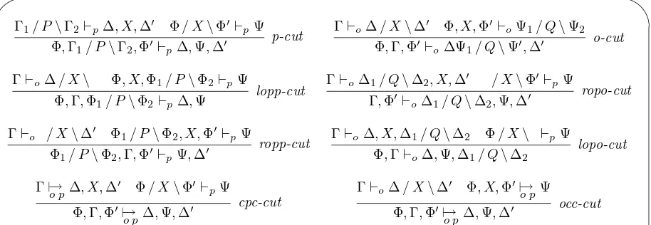
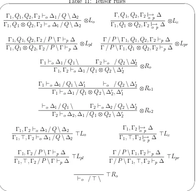
The logic has twenty four cut rules — although this may seem a lot, there is a simple underlying principle, which is we permit all possible well-typed, planar variants of the cut rule. As a single scheme, this would look something like this:
Γ⊢x ∆X∆′ ΦXΦ′ ⊢y Ψ ΦΓΦ′ ⊢z ∆Ψ∆′
where one of ∆,Φ must be empty, and one of ∆′,Φ′ must be empty (this is the planarity
condition). There are only six choices of the types of entailment ⊢x,⊢y,⊢z that are permitted by the typing, and with four alternatives for each, we end up with the twenty four variants. These are illustrated in Table 5, where we leave to the reader the task of implementing the planarity condition. The opp-cuts are given in two versions, each with two variants, because the cut is being made into one side of the context or the other—a similar division is made for the dual opo-cuts.
Notice that all these rules preserve the basic duality of this logic obtained by swapping the direction of the sequents, exchanging player for opponent and products for sums. Furthermore, we have represented this duality in the left column right column symmetry in the table. Recall also that the exchange rule can be assumed, in which case the phrases are to be regarded as bags of propositions.
4.2. Polarized polycategories.Corresponding to the logic of polarized cut above is its categorical proof theory which is the notion of a polarized polycategory. In addition polarized polycategories, like polycategories, have a term logic which consists of polarized circuits. The purpose of this section is to introduce these ideas.
A polarized polycategory X consists of polycategories Xo and Xp as well as a poly-module Xb. Each polyarrow in Xo is of the form
Table 5: General cut rules
✬
✫
✩
✪
Γ1/ P\Γ2⊢p∆, X,∆′ Φ/ X\Φ′ ⊢pΨ
Φ,Γ1/ P\Γ2,Φ′ ⊢p∆,Ψ,∆′
p-cut Γ⊢o∆/ X\∆
′ Φ, X,Φ′ ⊢oΨ1/ Q\Ψ2
Φ,Γ,Φ′⊢o∆Ψ1/ Q\Ψ′,∆′ o-cut
Γ⊢o∆/ X\ Φ, X,Φ1/ P\Φ2⊢pΨ
Φ,Γ,Φ1/ P\Φ2⊢p∆,Ψ
lopp-cut Γ⊢o∆1/ Q\∆2, X,∆
′ / X\Φ′ ⊢pΨ
Γ,Φ′ ⊢
o∆1/ Q\∆2,Ψ,∆′
ropo-cut
Γ⊢o / X\∆′ Φ1/ P\Φ2, X,Φ′⊢pΨ
Φ1/ P\Φ2,Γ,Φ′ ⊢pΨ,∆′
ropp-cut Γ⊢o∆, X,∆1/ Q\∆2 Φ/ X\ ⊢pΨ
Φ,Γ⊢o∆,Ψ,∆1/ Q\∆2
lopo-cut
Γ→o
p ∆, X,∆′ Φ/ X\Φ′⊢pΨ Φ,Γ,Φ′
o →
p∆,Ψ,∆′
cpc-cut
Γ⊢o∆/ X\∆′ Φ, X,Φ′
o →
pΨ Φ,Γ,Φ′
o →
p∆,Ψ,∆′
occ-cut
where in each rule where they appear, one of ∆,Φ is empty, and one of ∆′,Φ′ is empty.
having a sequence of objects Γ from Xo as its domain, and a sequence of objects all but one of which are from Xp as its codomain, with in addition one identified (“active”, or “in focus”) object from Xo: ∆,∆′ from Xp, Y from Xo. This collection of arrows must contain an “identity” arrow Y o// / Y \ for each object Y of Xo.
Dually, each polyarrow in Xp is of the form Γ/ X\Γ′ p// ∆
having a sequence of objects all but one of which are from Xo as its domain, with in addition one identified (“active”, or “in focus”) object from Xp in the domain, and a sequence of objects fromXp as its codomain: Γ,Γ′ fromXo,X,∆ fromXp. This collection of arrows must contain an “identity” arrow / X\ p// X for each object X of Xp.
We shall usually omit the subscripts on arrows in Xo,Xp, when the context makes them unnecessary.
Each polyarrow in the polymodule has the form Γ //∆
having a sequence Γ of objects from Xo in the domain and a sequence ∆ of objects from Xp in the codomain.
These arrows may be composed in four ways, essentially as given by the twenty-four cut rules of game logic above. This may seem rather intimidating, but in essence the idea is quite simple: each ofXoandXpallow composition much as ordinary polycategories do, but given the non-commutative nature of these sequents, there are minor variants caused by the placement of the active object in the sequents. In addition, Xo acts on
b
types of arrows.
Γ f //∆X∆′ ΦXΦ′ g //Ψ ΦΓΦ′ f;g //∆Ψ∆′
where one of ∆,Φ is empty, and one of ∆′,Φ′ is empty. (This condition is referred to as
the “planarity condition”.) In terms of circuits, this is even simpler; it is the usual circuit cut (just join two wires which bear the same label), with the understanding now that the joined wires are of the same type (player or opponent, “solid” or “dotted”).
There are “standard” unit and associativity conditions, analogous to those for ordinary polycategories. For simplicity, we illustrate these rules with “generic” versions. In these, we suppress the notation for which type of arrows are involved, where the composition (or cut) takes place, and so which type of composition or cut is involved; the reader is supposed to imagine all possible “well-typed” versions of these rules.
Recall that our compositions or cuts are supposed to be planar; we represent that by the convention that in these rules, an expression “∆|Γ” is to be understood as the trivial concatenation of a sequence and an empty sequence, the assumption being that one of ∆,Γ is empty.
(1)[idL] Γ1 f //Γ2, A,Γ3 = Γ1
f
/
/Γ2, A,Γ3 A iA //A Γ1 f;iA //Γ2, A,Γ3
(2)[idR] Γ1, A,Γ2 f //Γ3 = A
iA
/
/A Γ1, A,Γ2 f //Γ3 Γ1, A,Γ2 iA;f //Γ3
(3)[assoc]
Γ1 f //Γ2, A,Γ3 ∆1, A,∆2 g //∆3, B,∆4
∆1,Γ1,∆2 f;g //Γ2,∆3, B,∆4,Γ3 Φ1, B,Φ2 h //Φ3 Φ1,∆1,Γ1,∆2,Φ2
(f;g) ;h
/
/Γ2,∆3,Φ3,∆4,Γ3
=
∆1, A,∆2 g //∆3, B,∆4 Φ1, B,Φ2 h //Φ3 Γ1 f //Γ2, A,Γ3 Φ1,∆1, A,∆2,Φ2 g;h //∆3,Φ3,∆4
Φ1,∆1,Γ1,∆2,Φ2 f; (g;h) //Γ2,∆3,Φ3,∆4,Γ3
(4)[inter1]
Γ1 f //Γ2, A,Γ3 Φ1, A,Φ2, B,Φ3 h //Φ4 ∆1 g //∆2, B,∆3 Φ1,Γ1,Φ2, B,Φ3 f;h //Γ2,Φ4,Γ3
Φ1,Γ1,Φ2,∆1,Φ3 g; (f;h) //∆2 |Γ2,Φ4,∆3 |Γ3
=
∆1 g //∆2, B,∆3 Φ1, A,Φ2, B,Φ3 h //Φ4 Γ1 f //Γ2, A,Γ3 Φ1, A,Φ2,∆1,Φ3 g;h //∆2,Φ4,∆3
(5)[inter1]
Γ1 f //Γ2, A,Γ3, B,Γ4 ∆1, A,∆2 g //∆3
∆1,Γ1,∆2 f;g //Γ2,∆3,Γ3, B,Γ4 Φ1, B,Φ2 h //Φ3 Φ1 |∆1,Γ1,Φ2 |∆2 (f;g) ;h //Γ2,∆3,Γ3,Φ3,Γ4
=
Γ1 f //Γ2, A,Γ3, B,Γ4 Φ1, B,Φ2 h //Φ3
Φ1,Γ1,Φ2 f;h //Γ2, A,Γ3,Φ3,Γ4 ∆1, A,∆2 g //∆3 Φ1 |∆1,Γ1,Φ2 |∆2 (f;h) ;g //Γ2,∆3,Γ3,Φ3,Γ4
This completes the definition of a polarized polycategory.
4.3. Polarized proof circuits.There is a very convenient visual term logic for po-larized polycategories in which the identities become topological identities. This is a generalization of the proof circuits introduced in [BCST96]. The generalization requires that one labels wires not only by their type but also by the category in which their type lives (i.e. the opponent or player category). Following the convention that hollow nodes represent opponent positions and solid nodes represent player positions, we shall draw “opponent wires” as dotted and “player wires” as solid. All wires and nodes are supposed to be labelled, although when unnecessary for the purpose at hand, we shall often drop the labels to make the drawing clearer.
☞ ☞ ☞
▲ ▲
▲ ☞
☞ ☞
▲ ▲
▲
A polyarrow inXo
☞ ☞ ☞
▲ ▲
▲ ☞
☞ ☞
▲ ▲
▲
A polyarrow in Xp
☞ ☞ ☞
▲ ▲
▲ ☞
☞ ☞
▲ ▲
▲
A polyarrow in Xb
☞
These circuits allow us to build polarized polycategories based on a given set of polar-ized types (that is a set of opponent types and a set of player types) and a set of polarpolar-ized components. The components must each be provided with a type which is a polarized sequent. This data we call a polarized polygraph G and we can build from it a polarized polycategoryF(G) with the same types. We do this by building the polyarrows, which we call polarized proof circuits, inductively from the polarized polygraph by cutting together polarized proof circuits starting with components and wires (the identity maps). Circuit equivalence is then given by topological equivalence of the circuits.
Note that each proof circuit must have an explicit inductive construction fromGusing cuts. It is well known that this is equivalent to requiring the result be a planar tree, and indeed in testing that a circuit is a planar tree it is possible to take a rewriting approach (this is often called sequentialization) in which one performs cuts to build larger and larger subcircuits which are proofs. The process is confluent and is successful if the whole circuit is collected [BCST96].
Every polarized polycategory has an obvious underlying polarized graph and this ex-tends to a functor U:PolPolycat //PolyGraph. We have:
4.3.1. Proposition.The underling functor U:PolPolycat //PolyGraph has a left
adjoint which associates to each polarized polygraph its polarized polycategory of polarized proof circuits.
The proof of this involves realizing that the notion of topological equivalence is exactly what is given by the associativity and interchange equations of polarized polycategories. Before looking at some basic examples of polarized polycategories it is worth making some observations about these free polarized polycategories and their relationship to free (unpolarized) polycategories which are constructed in the same manner, see [BCST96].
We shall say a polyarrow is focused in case its type is a player or opponent sequent; it is unfocused otherwise. We start by observing:
4.3.2. Lemma.
1. A focused polyarrow g ∈F(G) contains no unfocused components.
2. An unfocused polyarrow f ∈F(G) must contain exactly one unfocused component;
Proof. 1. A focused polyarrow could be a wire or a single component. If it is not one of these it is a polarized cut of two subcircuits. However, note that the focused edge is attached to one of these subcircuits, which means it is focused. Furthermore, the (therefore unfocused) cut edge of this circuit is forced to be a focused edge of the other subcircuit. This means that subcircuits are focused so by induction all subcircuits are focused.
2. If f is unfocused it cannot be a wire. If it consists of a single component we are done. If it is the cut of two subcircuits whichever polarization the cut wire is forces one circuit to be focused (and so by the above has no unfocused components) and the other to be unfocused and thus have, by induction, exactly one unfocused component.
In the terminology of processes, what this is saying is that in a polarized system there can only be one process which is sending a message. This means that the message passing can be regarded as completely sequential. So this does not provide a model of true concurrency.
This observation has some rather surprising formal consequences:
4.3.3. Corollary.If G is a polygraph with no unfocused components then F(G) has no mixed polyarrows (i.e. the module is empty).
4.3.4. Corollary.In the free polycategory:
1. For each polyarrow and focused polarization of its type, there is exactly one polar-ization of the polyarrow to achieve that polarized type;
2. For each polyarrow and unfocused polarization of its type there are exactly n polar-izations of the polyarrow, where n is the number of components in the polyarrow.
Proof.1. The decomposition of the polyarrow using cuts determines the polarization of subcircuits until the components are reached.
2. Exactly one component must be of mixed polarity; however, we can choose that component freely. On the other hand, once the component is chosen the rest of the typing is determined.
As an illustration, consider the following simple circuit.
A ⊢f X X, B ⊢g A, B ⊢f;g
g f
❉ ❉❉ ✆✆
✆✆ ✆✆
A B
X
There are only two ways the conclusion may be polarized as a focused sequent: because of the empty conclusion⊥ of f ;g (which must be typed P), the sequent must have type
P, which can be done two ways, / A\B ⊢p ⊥orA / B\ ⊢p ⊥. According to the Corollary, for each of these there can be only one way to type the components f, g to achieve the polarization. Indeed, the typing must be done so that exactly one of AorB is of typeP, and X must be of the same type as A. This gives these two focused derivations:
A⊢p X / X\B ⊢p
A, B ⊢p and
A ⊢oX X / B\ ⊢p A, B ⊢p
In circuits:
g f
❉ ❉❉
A B
X
g f
✆✆ ✆✆
✆✆
A B
X
If we typef ;gas mixed (unfocused), then there are two typings off, gthat accomplish this (note n = 2 in this example), one in whichX isO, the other in which it is P:
A ⊢o/ X\ X, B o→p A, B o→
p and
A o→
p X / X\B ⊢p A, B o→
In circuits:
g f A B
X
g f
❉ ❉❉
A B
X
4.4. Examples. There are several examples of polarized polycategories, starting with our main example.
4.4.1. Example.Our main example of a polarized polycategory, of course, is derived from the combinatorial AJ games with which we started. To obtain a polarized polycategory from them, we take the same objects as before, but must modify the arrows somewhat to get polyarrows of the appropriate sorts. We shall use the notation from before, adapted to the “multi-channel” context; so each position (“channel”) in a polyarrow will be given a “channel name”, which will be carried through the formation of new polyarrows. Note that just as before, this notation can also be used to derive a term calculus for polarized polycategories.
[Opponent polyarrows:]
α
b1 7→ h1 · · · bm 7→ hm
: Γ //∆/ α: (b1:P1, . . . , bm:Pm)\∆′
where each hi: Γ //∆, α:Pi,∆′ is a module polyarrow, and α labels one of the channels.
[Module polyarrows:] These are either of the form −
→α[ak]·g: Γ //∆/ α:{a1:O1, . . . , an:On} \∆′
wherek∈ {1, . . . , n},g: Γ //∆/ α:Ok\∆′ is an opponent polyarrow, andαlabels one of the channels, or
←α−[b
k]·f: Γ, α: (b1:P1, . . . , bn:Pn),Γ′ //∆
wherek ∈ {1, . . . , n},f: Γ/ α:Pk\Γ′ //∆ is a player polyarrow, andαis a channel
label.
[Player polyarrows:]
α
a1 7→ h1 · · · am 7→ hm
: Γ/ α:{a1:O1, . . . , am:Om} \Γ
′ //∆
As an example of such a polyarrow, the following is a module polyarrow. (We’ve only labeled plays that enter into the construction of the arrow, for clarity.)
←−
There is a pleasant interpretation of these polyarrows. A polyarrow is a process which we may view as a person, say Mike, sitting in an office with a number of telephones which are directly connected to other offices: some of these telephones are white (and connect to white phones) and some are black (and connect to black phones) . When Mike is a module polyarrow he may pick up any of the telephones and send a message to the person in the office to which that phone is connected. However, Mike can only hold one telephone at a time and, if he sends a message to Mary who is sitting in another office, he must then hold this line until he receives a response from Mary. When he is holding the line in this manner he is “focused” on Mary and is either an opponent or a player polyarrow depending (respectively) on whether the phone he is holding is white or black. Only when Mike has received a response from Mary is he free to put down Mary’s phone. At that stage Mike becomes a module polyarrow again and can pick up any of his phones again. In the example above the conversation went as follows: Mike starts by picking up the white phone, labelled β, and sends the message x to Mary. He then awaits Mary’s response which could be, according to the preset protocol, either av or aw. When Mary responds with a v, Mike will pick up the black phone, labelledδ, and send the messagea to Bob. Mike will not expect a response from Bob because his task will be complete and he will never put down the phone. On the other hand, if Mary responds with a w, Mike will pick up the black phone labelled ǫ and send the message d to Martha: he will not expect a response from Martha and so be left holding this phone.
4.4.2. Example. Spans of sets and partial maps form a polarized polycategory X, in the following manner. The objects of Xo,Xp and Xb are all sets; arrows in Xo are spans Q1 oo · // //Q2 where the right leg is mono, arrows “P1 //P2” in Xp are the dual,
sequent would look like this, with m monic.
We may think of this arrow in relational database terms as a table with a specified key. Cut is given by pullback, and it is a standard fact that pullbacks will preserve monics, so the typing is respected.
4.4.3. Example. The next example uses the notion of a linear functor between two polycategories; these are introduced in [CS99, CKS]. Let F = (F⊗, F⊕):A //B be a
linear functor; then we can obtain a polarized polycategory XF from F as follows. The objects of XF o are pairs (A,) for A an object of A; we think of such an object as the object F⊗(A). Objects of XF p are pairs (A,), which we shall think of as F⊕(A). Note
that equality of objects is determined by equality in A, not by equality of images in B. An O-sequent, which we can think of as
F⊗(A1),· · ·, F⊗(An) //F⊕(A′1),· · ·, F⊕(Ai′−1)/ F⊗(A)\F⊕(A′i+1),· · ·, F⊕(A′m)
is the F⊗ image (we called this an F⊗ functor box in [CS99, CKS]) of an A sequent
A1,· · ·, An //A′1,· · ·, A′i−1, A, A′i+1,· · ·, A′m. Dually, a P-sequent is theF⊕ image of an
A sequent. Cross (mixed) sequents are arbitrary B sequents of the form F⊗(A1),· · ·, F⊗(An) //F⊕(A
′
1),· · ·F⊕(A
′
m)
Composition (cut) is given as follows. “Pure” (OorP) sequents compose by composition inA (taking the appropriate F⊗ or F⊕ image, as determined by the typing); composition
(cut) with a cross sequent is just composition inB. This is well typed since pure sequents compose with pure sequents to give pure sequents, but composition with a cross sequent gives a cross sequent. The identities for a polycategory are then trivially induced by those identities in the underlying A, B.
We remark here (for the experts) that hypercoherences may be seen as an instance of this example. We recall that a hypercoherence E may be regarded as a “hypergraph”, determined by a set |E| of “nodes” and a set Γ(E) of “hyperedges”, where a hyperedge is a finite non-empty set of nodes; Γ(E) is required to contain all singletons (which may be thought of as “loops”). These naturally form a categoryHC, in fact, a∗-autonomous category with products (and so coproducts); very roughly, maps may be thought of as relations mapping hyperedges to hyperedges, with the restriction that only loops may be mapped to loops. HC has a full subcategory HC+ of “hereditary” hypercoherences, i.e. those hypercoherences whose sets of hyperedges are “down-closed”, in the sense that ifu is a finite non-empty subset of a hyperedge, it also is a hyperedge. HC+ is a coreflective subcategory of HC; the right adjoint to the inclusion is ↓:HC //HC+, where ↓ E has the same nodes as E, but whose hyperedges are the down-closed hyperedges of E,