El e c t ro n ic
Jo ur
n a l o
f P
r o
b a b il i t y
Vol. 14 (2009), Paper no. 22, pages 569–593. Journal URL
http://www.math.washington.edu/~ejpecp/
Survival time of random walk in random environment
among soft obstacles
Nina Gantert
∗Serguei Popov
†Marina Vachkovskaia
‡Abstract
We consider a Random Walk in Random Environment (RWRE) moving in an i.i.d. random field of obstacles. When the particle hits an obstacle, it disappears with a positive probability. We obtain quenched and annealed bounds on the tails of the survival time in the general d-dimensional case. We then consider a simplified one-dimensional model (where transition probabilities and obstacles are independent and the RWRE only moves to neighbour sites), and obtain finer results for the tail of the survival time. In addition, we study also the “mixed" probability measures (quenched with respect to the obstacles and annealed with respect to the transition probabilities and vice-versa) and give results for tails of the survival time with respect to these probability measures. Further, we apply the same methods to obtain bounds for the tails of hitting times of Branching Random Walks in Random Environment (BRWRE).
Key words:confinement of RWRE, survival time, quenched and annealed tails, nestling RWRE, branching random walks in random environment.
AMS 2000 Subject Classification:Primary 60K37.
Submitted to EJP on June 9, 2008, final version accepted January 20, 2009.
∗CeNos Center for Nonlinear Science and Institut für Mathematische Statistik, Fachbereich Mathematik und Informatik,
Einsteinstrasse 62, 48149 Münster, Germany. e-mail:[email protected]
†Instituto de Matemática e Estatística, Universidade de São Paulo, rua do Matão 1010, CEP 05508–090, São Paulo SP,
Brasil. e-mail:[email protected], url:www.ime.usp.br/∼popov
‡Departamento de Estatística, Instituto de Matemática, Estatística e Computação Científica, Universidade de
1
Introduction and main results
Random walk and Brownian motion among random obstacles have been investigated intensively in the last three decades. For an introduction to the subject, its connections with other areas and an exposition of the techniques used, we refer to the book[8]. Usually, one distinguisheshard obstacles, where the particle is killed upon hitting them, andsoft obstacleswhere the particle is only killed with a certain probability. A typical model treated extensively in[8]is Brownian motion in a Poissonian field of obstacles. The following questions arise for this model: what is the asymptotic behaviour of the survival time? What is the best strategy of survival, i.e. what is the conditioned behaviour of the particle, given that it has survived until timen? An important role in answering these questions has been played by the concept of “pockets of low local eigenvalues” (again, we refer to [8] for explanations). A key distinction in random media is the difference between thequenched probabil-ity measure (where one fixes the environment) and theannealed probability measure (where one averages over the environment).
In this paper, we are considering a discrete model with soft obstacles where there are two sources of randomness in the environment: the particle has random transition probabilities (which are as-signed to the sites of the lattice in an i.i.d. way and then fixed for all times) and the obstacles are also placed randomly on the lattice and then their positions remain unchanged. We investigate the tails of the survival time. Similar questions have been asked in[1] for simple random walk. The “pockets of low local eigenvalues” are in our case “traps free of obstacles”: these are regions without obstacles, where the transition probabilities are such that the particle tends to spend a long time there before escaping. These regions are responsible for the possibility of large survival time. We as-sume that the environments (transition probabilities and obstacles) in all sites are independent and obtain quenched and annealed bounds on the tails of the survival time in the generald-dimensional case. We then consider a simplified one-dimensional model (where transition probabilities and ob-stacles are independent and the RWRE only moves to neighbour sites), and obtain finer results for the tail of the survival time. Having two sources of randomness in the environment, we study also the “mixed" probability measures (quenched with respect to the obstacles and annealed with respect to the transition probabilities and vice-versa) and give results for the tails of the survival time with respect to these probability measures. Further, we develop the analogy with the branching random walks in random environment (BRWRE) [4; 5], and provide quenched and annealed bounds for hitting times in the BRWRE model.
Now we define the model formally. Denote by e1, . . . ,ed the coordinate vectors, and letk · k1 and
k · k2 stand for the L1 and L2 norms in Zd respectively. The environment consists of the set of
transition probabilitiesω = (ωx(y), x,y ∈Zd), and the set of variables indicating the locations
of the obstacles θ = (θx, x ∈ Zd), where θx = 1{there is an obstacle inx}. Let us denote by
σx = (ωx(·),θx)the environment in x∈Zd, andσ= (ω,θ) = (σx, x ∈Zd)stands for the (global) environment. We suppose that jumps are uniformly bounded by some constantme, which means that
ωx(y) =0 ifkx−yk1>me. Let us denote byM the environment space where theσx are defined, i.e.
M =n (a(y))y∈Zd,b:a(y)≥0,∀y∈Zd,
X
y∈Zd
a(y) =1= X
y:kyk1≤me
We assume that (σx, x ∈Zd) is a collection of i.i.d. random variables. We denote by P the cor-responding product measure, and by E its expectation. In some cases these assumptions may be relaxed, see Remark 1.3 below.
Let
p=P[θ0=1]. We always assume 0<p<1.
Having fixed the realization of the random environmentσ, we now define the random walkξand
the random timeτ as follows. The discrete time random walk ξn starts from some z0 ∈Zd and
moves according to the transition probabilities
Pz0
σ[ξn+1=x+y |ξn= x] =ωx(y). Here Pz0
σ stands for the so-called quenched probability (i.e., with fixed environment σ) and we
denote byEz0
σ the corresponding expectation. Usually, we shall assume that the random walk starts
from the origin, so thatz0=0; in this case we use the simplified notationsPσ,Eσ.
Fixr∈(0, 1)and letZ1,Z2, . . . be a sequence of i.i.d. Bernoulli random variables withPσ[Zi =1] = r. Denote byΘ ={x ∈Zd: θx =1}the set of sites where the obstacles are placed. Let
τ=min{n: ξn∈Θ,Zn=1}.
Intuitively, when the RWRE hits an obstacle, it “disappears” with probabilityr, andτis the survival time of the particle.
We shall also consider the annealed probability lawPz0=P×Pz0
σ[·], and the corresponding
expecta-tionEz0=EEz0
σ. Again, when the random walk starts from the origin, we use the simplified notations P,E.
Throughout this paper we suppose that that the environment σsatisfies the following two
condi-tions.
Condition E.There existsǫ0>0 such thatωx(e)≥ǫ0 for alle∈ {±ei, i=1, . . . ,d},P-a.s.
For(ω,θ)∈ M, let
∆ω=X
y
yω(y) (1)
be the drift ofω.
Condition N.We have
P[θ0=0,∆ω·a>0]>0 for alla∈Rd\ {0}.
Our goal is to study the quenched and annealed tails of the distribution of τ: Pσ[τ > n] and P[τ >n].
First, we formulate the results on the tails ofτin thed-dimensional case under the above assump-tions:
Theorem 1.1. For all d≥1there exist Kia(d)>0, i=1, 2, such that for all n
P[τ >n]≤exp(−Ka 1(d)ln
dn), (2)
and
P[τ >n]≥exp(−Ka 2(d)ln
dn). (3)
Theorem 1.2. For d ≥1there exist Kiq(d)> 0, i =1, 2, 3, 4(also with the property Kqj(1) <1for j=2, 4), such that forP-almost allσthere exists n0(σ)such that for all n≥n0(σ)we have
Pσ[τ >n]≤exp −K
q
1(d)nexp(−K
q
2(d)ln
1/dn), (4)
and
Pσ[τ >n]≥exp −K
q
3(d)nexp(−K
q
4(d)ln
1/dn). (5)
In fact (as it will be discussed in Section 2) the original motivation for the model of this paper came from the study of the hitting times for branching random walks in random environment (BRWRE), see [4]. The above Theorem 1.1 has direct counterparts in [4], namely, Theorems 1.8 and 1.9. However, the problem of finding upper and lower bounds on the quenched tails of the hitting times was left open in that paper (except for the case d = 1). Now, Theorem 1.2 of the present paper allows us to obtain the analogous bounds also for the model of [4]. The model of [4] can be described as follows. Particles live inZd and evolve in discrete time. At each time, every particle
in a site is substituted by (possibly more than one but at least one) offspring which are placed in neighbour sites, independently of the other particles. The rules of offspring generation (similarly to the notation of the present paper, they are given byωx at sitex) depend only on the location of the particle. Similarly to the situation of this paper, the collectionωof those rules (theenvironment) is
itself random, it is chosen in an i.i.d. way before starting the process, and then it is kept fixed during all the subsequent evolution of the particle system. We denote byωa generic element of the set of all possible environments at a given point, and we distinguishω with branching (the particle can be replaced with several particles) andωwithout branching (the particle can only be replaced with exactly one particle). The BRWRE is called recurrent if for almost all environments in the process (starting with one particle at the origin), all sites are visited (by some particle) infinitely often a.s. Using the notations of[4](in particular,Pωstands for the quenched probability law of the BRWRE),
we have the following
Proposition 1.1. Suppose that the BRWRE is recurrent and uniformly elliptic. Let T(0,x0) be the hitting time of x0 for the BRWRE starting from0. Then, there existKb
q
i(d)>0, i=1, 2, 3, 4, such that for almost all environmentsω, there exists n0(ω)such that for all n≥n0(ω)we have
Pω[T(0,x0)>n]≤exp −Kb
q
1(d)nexp(−Kb
q
2(d)ln
1/dn). (6)
Now, letG be the set of allωwithout branching. Suppose that it has positive probability and the origin belongs to the interior of the convex hull of{∆ω:ω∈ G ∩suppP}, where∆ω is the drift from a site
with environmentω. Suppose also that there isǫˆ0 such that
PPω[total number of particles at time 1 is 1]≥ǫˆ0
i.e., for almost all environments, in any site the particle does not branch with uniformly positive proba-bility. Then
Pω[T(0,x0)>n]≥exp −Kb
q
3(d)nexp(−Kb
q
4(d)ln
1/dn). (7)
Now, we go back to the random walk among soft obstacles. In the one-dimensional case, we are able to obtain finer results. We assume now that the transition probabilities and the obstacles are independent, in other words, P = µ⊗ν, where µ,ν are two product measures governing, respectively, the transition probabilities and the obstacles. We further assumeme=1 and we denote
ω+x =ωx(+1)andω−x =1−ω
+
x =ωx(−1). Condition N is now equivalent to inf{a: µ(ω+0 ≤a)>0}<1/2,
sup{a: µ(ω+0 ≥a)>0}>1/2, (8) i.e., the RWRE is strictly nestling. Let
ρi= ω
− i
ω+i , i∈Z. (9)
Defineκℓ=κℓ(p)such that
E
1
ρκℓ 0
= 1
1−p (10)
andκr=κr(p)such that
E(ρκr
0 ) =
1
1−p (11)
Due to Condition N, since 0<p<1,κℓandκrare well-defined, strictly positive and finite. Indeed, to see this forκr, observe that for the function f(x) =E(ρ0x)it holds that f(0) =1, f(x)→ ∞as x → ∞, and f is convex, so the equation f(x) =uhas a unique solution for anyu>1. A similar argument implies thatκℓ is well-defined.
We now are able to characterize the quenched and annealed tails ofτin the following way:
Theorem 1.3. For d =1
lim n→∞
lnP[τ >n]
lnn =−(κℓ(p) +κr(p)). (12)
Theorem 1.4. For d =1
lim n→∞
ln(−lnPσ[τ >n])
lnn =
κℓ(p) +κr(p) 1+κℓ(p) +κr(p)
P-a.s. (13)
In our situation, besides the quenched and the annealed probabilities, one can also consider two “mixed” ones: the probability measurePωz=ν×Pσz which is quenched inωand annealed inθ and
the probability measurePθz=µ×Pσz which is quenched inθ and annealed inω. Again, we use the
simplified notationsPω=Pω0, Pθ =Pθ0.
Let
β0=inf{ǫ: µ[ω+0 < ǫ]>0}
β1=1−sup{ǫ: µ[ω+0 > ǫ]>0}.
Due to (8) we haveβ0 < 1/2, β1 <1/2. Then, we have the following results about the “mixed”
Theorem 1.5. For d =1,
These random variables have the following properties: there exists a family of nondegenerate random variables(Ξ(ǫ),ǫ≥0)such that
Remark 1.1. In fact, a comparison with Theorems 1.3 and 1.4 of[7]suggests that
lim sup and, in particular, forµ-almost allωand some positive constants C1,C2,
lim sup
However, the proof of (19)–(21) would require a lengthy analysis of fine properties of the potential V (see Definition 3.1 below), so we decided that it would be unnatural to include it in this paper.
Remark 1.2. It is interesting to note that r does only enter the constants, but not the exponents in all these results.
2
Proofs: multi-dimensional case
In this section, we prove Theorems 1.1 and 1.2. In fact, the ideas we need to prove these results are similar to those in the proofs of Theorems 1.8 and 1.9 of[4]. In the following, we explain the relationship of the discussion in[4]with our model, and give the proof of Theorems 1.1 and 1.2, sometimes referring to[4]for a more detailed account.
Proof of Theorems 1.1 and 1.2.The proof of (2) follows essentially the proof of Theorem 1.8 of[4], where it is shown that the tail of the first hitting time of some fixed site x0 (one may think also of
the first return time to the origin) can be bounded from above as in (2). The main idea is that, as a general fact, for any recurrent BRWRE there are the so-calledrecurrent seeds. These are simply finite configurations of the environment, where, with positive probability, the number of particles grows exponentially without help from outside (i.e., suppose that all particles that step outside this finite piece are killed; then, the number of particles in the seed dominates a supercritical Galton-Watson process, which explodes with positive probability). Then, we consider an embedded RWRE, until it hits a recurrent seed and the supercritical Galton-Watson process there explodes (afterwards, the particles created by this explosion are used to find the site x0, but here this part is only needed for Proposition 1.1).
So, going back to the model of this paper, obstacles play the role of recurrent seeds, and the mo-mentτwhen the event{ξn∈Θ,Zn =1}happens for the first time is analogous to the moment of the first explosion of the Galton-Watson process in the recurrent seed. To explain better this analogy, consider the following situation. Suppose that, outside the recurrent seeds there is typically a strong drift in one direction and the branching is very weak or absent. Then, the qualitative behaviour of the process is quite different before and after the first explosion. Before, we typically observe very few (possibly even one) particles with more or less ballistic behaviour; after, the cloud of particles starts to grow exponentially in one place (in the recurrent seed where the explosion occurs), and so the cloud of particles expands linearly in all directions. So, the first explosion of one of the Galton-Watson processes in recurrent seeds marks the transition between qualitatively different behaviours of the BRWRE, and thus it is analogous to the momentτof the model of the present paper.
First, we prove (2) ford≥2. For anya∈Z, defineKa = [−a,a]d. Choose anyα <(lnǫ−1 0 )−1 (ǫ0
is from Condition E) and define the event
Mn={σ: for any y ∈ Kmne there existsz∈Θsuch thatky−zk1≤αlnn}
(recall thatme is a constant such thatωx(y) =0 ifkx−yk>me, introduced in Section 1). Clearly, we have ford≥2
P[Mnc]≤C1ndexp(−C2lndn). (22)
Now, suppose thatσ ∈Mn. So, for any possible location of the particle up to time n, we can find
a site with an obstacle which is not more than αlnnaway from that location (in the sense of L1 -distance). This means that, on any time interval of lengthαlnn, the particle will disappear (i.e.,τ
is in this interval if the particle has not disappeared before) with probability at least rǫ0αlnn, where
the interval[0,n], so
Pσ[τ >n]≤(1−rǫ0αlnn)
n
αlnn
≤exp
− C3n
1−αlnǫ−01
lnn
. (23)
Then, from (22) and (23) we obtain (recall thatαlnǫ−01<1)
P[τ >n]≤exp
−C3n
1−αlnǫ−1 0
lnn
+C1ndexp(−C2lndn),
and hence (2).
Let us now prove (4), again for the cased≥2. Abbreviate byℓd= 2 d
d! the volume of the unit sphere
inRd with respect to theL1 norm, and letq=P[θ0=0] =1−p. Choose a large enoughαbin such
a way thatℓdαbdlnq−1>d+1, and define
b
Mn={σ: for any y∈ K
e
mnthere existsz∈Θ
such thatky−zk1≤αbln1/dn}.
By a straightforward calculation, we obtain ford≥2
P[Mbnc]≤C4ndn−ℓdαb
dlnq−1
. (24)
Using the Borel-Cantelli lemma, (24) implies that for P-almost allσ, there existsn0(σ)such that σ∈Mbn for alln≥n0(σ).
Consider now an environmentσ∈Mbn. In such an environment, in the L1-sphere of sizenaround
the origin, any L1-ball of radiusαbln1/dncontains at least one obstacle (i.e., a point fromΘ). This means that, in any time interval of lengthαbln1/dn, the particle will disappear with probability at leastrǫαbln1/dn
0 , where, as before,ǫ0 is the constant from the uniform ellipticity Condition E. There
are n
b
αln1/dn such intervals on[0,n], so
Pσ[τ >n]≤(1−rǫbαln 1/dn
0 )
n
b
αln1/d n,
which gives us (4) in dimensiond≥2.
Now, we obtain (2) and (4) in the one-dimensional case. Since the environment is i.i.d., there existγ1,γ2>0 such that for any intervalI⊂Z,
P[|I∩Θ| ≥γ1|I|]≥1−e−γ2|I|. (25)
We say that an intervalI isnice, if it contains at leastγ1|I|sites fromΘ.
Define
h(σ) =min{m: all the intervals of lengthk≥m
intersecting with[−eγ2k/2,eγ2k/2]are nice}.
It is straightforward to obtain from (25) that there existsC5>0 such that
In particular,h(σ)is finite forP-almost allσ.
Now, define the event F ={maxs≤n|ξs| ≤ na}, wherea=
γ2 4 lnǫ−1
0
. By Condition E, during any time
interval of length lnn
2 lnǫ−1 0
the random walk completely covers a space interval of the same length with probability at least
2 lnǫ0−1, and consider such an interval successful if the random walk completely
covers a space interval of the same length: we then have 2nlnǫ−
1 0
lnn independent trials with success probability at leastn−1/2, and then one can use Chernoff’s bound for Binomial distribution (see e.g. inequality (34) of[4]). Hence we obtain for suchσ
fork≥1. Defining also the sequence of events
Dk={there existst∈[tk,tk+me−1]such thatξt∈ΘandZt =1},
and we obtain (4) from (27) and (29) (notice that in the one-dimensional case, the right-hand side of (4) is of the form exp(−K1q(1)n1−K2q(1))). Then, the annealed upper bound (2) for d =1 follows
from (4) and (26).
(iii) there exists a1 >0 such that for anyz ∈Ui and anyσ= (ω,θ)∈Γi we have z·∆ω<−a1 (recall Condition N).
Intuitively, this collection will be used to construct (large) pieces of the environment which are free of obstacles (item (i)) and have the drift pointing towards the center of the corresponding region (item (iii)). The cost of constructing piece of environment of sizeN (i.e., containing N sites) with such properties does not exceedpN1 (item (ii)).
Consider anyz∈Zd,B⊂Zd and a collectionH= (Hx ⊆ M,x∈B); let us define
S(z,B,H) ={σ:σz+x ∈Hx for allx ∈B}.
In[4], onS(z,B,H)we said that there is an(B,H)-seed inz; for the model of this paper, however, we prefer not to use the term “seed”, since the role seeds play in[4]is quite different from the use of environments belonging toS(z,B,H) here. Take G(n)={y ∈Zd :kyk2 ≤ulnn}, whereuis a
(large) constant to be chosen later. Let us define the setsH(xn),x ∈G(n)in the following way. First, putH0(n)= Γ1; for x 6=0, leti0 be such that kxxk ∈Ui0 (note that i0 is uniquely defined), then put
H(xn)= Γi
0. Clearly, for any y ∈Z
d
P[S(y,G(n),H(n))]≥p(12u)dlndn. (30)
Denote
bp= sup y:kyk1≤me
Pσy[ξhitsZ
d
\G(n)before 0].
As in [4] (see the derivation of (42) there), we obtain that there exist C9,C10 such that for all
σ∈ S(0,G(n),H(n))we have
b p≤ C9
nC10u. (31)
So, chooseu> C1
10, then, on the event that
σ∈ S(0,G(n),H(n)), (31) implies that
Pσ[ξi∈G(n)for alli≤n]≥(1−bp)n≥C11 (32)
(if the random walk hits the origin at least ntimes before hittingZd\G(n), thenξi ∈G(n)for all i≤n). SinceG(n)is free of obstacles, we obtain (3) from (30) and (32).
Now, it remains to prove (5). Define
b
G(n)={y ∈Zd:kyk2≤vln1/dn},
and let Hb(n) = (Hb(xn),x ∈Gb(n)) be defined in the same way as H(n) above, but with Gb(n) instead ofG(n). Analogously to (30), we have
P[S(y,Gb(n),Hb(n))]≥p1(2v)dlnn=n−(2v)dlnp−11. (33)
Choosev in such a way that b0:= (2v)dlnp1−1<d/2(d+1). Then, it is not difficult to obtain (by
dividingKp
n intoO(nd(
1
2−b0))subcubes of linear sizeO(nb0)) that
Ph [
z∈Kpn
S(z,Gb(n),Hb(n)) i
Using the Borel-Cantelli Lemma,P-a.s. for allnlarge enough we have
σ∈ [
z∈Kpn
S(z,Gb(n),Hb(n)).
Denote byTB the first hitting time of a setB⊂Zd:
TB=inf{m≥1 :ξm∈B},
and writeTa=T{a}for one-point sets. Next, forσ∈ S(0,Gb(n),Hb(n))we are going to obtain an upper bound forqx :=Pσx[ξhitsZd\Gb(n)before 0] =Pσx[T0>TZd\Gb(n)], uniformly inx∈Gb(n). To do this, note that there are positive constantsC13,C14such that, abbreviating B0 ={x ∈Zd :kxk2 ≤C13},
the process exp(C14kξm∧TB0k2)is a supermartingale (cf. the proof of Theorem 1.9 in[4]), i.e.,
Eσ exp(C14kξ(m+1)∧TB0k2)|ξj∧TB0,j≤m
≤exp(C14kξm∧TB0k2)
for allm. Denote
e
G(n)={x∈Zd:kxk2≤vln1/dn−1}.
For any x ∈Ge(n)and y ∈Zd\Gb(n), we havekxk2 ≤ kyk2−1, soeC14kxk2 ≤e−C14eC14kyk2. Keeping
this in mind, we apply the Optional Stopping Theorem to obtain that, for anyσ∈ S(0,Gb(n),Hb(n)),
qxexp(C14vln1/dn)≤exp(C14kxk2)≤e−C14exp(C
14vln1/dn),
so qx ≤ e−C14 for all x ∈ Ge. Now, from any y ∈ Gb(n)\Ge(n) the particle can come to Ge(n) in a
fixed number of steps (at most pd+1) with uniformly positive probability. This means that, on
S(0,Gb(n),Hb(n)), there exists a positive constantC15>0 such that for all x∈Gb(n)
Pσx[T0<TZd\Gb(n)]≥C15. (35)
Then, analogously to (31), onS(0,Gb(n),Hb(n))we obtain that, for all y such thatkyk1≤me
Pσy[ξhitsZ
d
\Gb(n)before hitting 0]≤ C16
ln1/dn.
So, using (35) onS(0,Gb(n),Hb(n))we obtain that there areC17andC18such that for allx ∈Gb(n)
Pσx[TZd\Gb(n)≥exp(C17ln1/dn)]≥C18. (36)
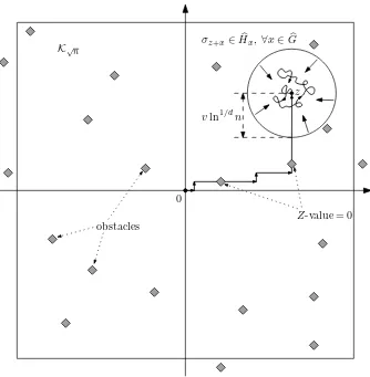
Then, we use the following survival strategy of the particle (see Figure 1): provided that the event
S(z,Gb(n),Hb(n)) occurs for some z ∈ Kpn, first the particle walks there (using, for instance, the shortest possible path) without disappearing in an obstacle; this happens with probability at least
(ǫ0(1−r))d
p
n. Then, it will spend time
n=exp(C17ln1/dn)×nexp(−C17ln1/dn)
inz+Gb(n)with probability at leastCnexp(−C17ln1/dn)
18 , so
Pσ[τ >n]≥(ǫ0(1−r))d
pn
Cnexp(−C17ln1/dn)
z
0 K√n
σz+x∈Hbx, ∀x∈Gb
vln1/dn
obstacles
Z-value = 0
and this gives us (5).
Proof of Proposition 1.1. Now, we explain how to obtain Proposition 1.1. To prove (6), we proceed as in the proof of (4). As noted in the beginning of this section, the disappearing of the particle in an obstacle is analogous to starting an exploding Galton-Watson process in a recurrent seed. Denote by Te the moment when this happens, i.e., at leasteC19k new particles are created in this recurrent
seed by timeTe+k. Thus, one can obtain a bound of the form
Pω[Te>n]≤exp −C20nexp(−C21ln1/dn)
.
Then, using the uniform ellipticity, it is straightforward to obtain that, waitingC22ntime units more
(with large enoughC22), one of the newly created (in this recurrent seed) particles will hit x0 with
probability at least 1−e−C23n, and this implies (6).
To show (7), we note that, analogously to the proof of (5) that we are able to create a seed which is free of branching sites of diameterC24ln1/dn, which lies at distanceO(pn)from the origin. Then,
the same idea works: the initial particle goes straight to the seed without creating new particles, and then stays there up to timen. The detailed proof goes along the lines of the proof of (5) only with notational adjustments.
3
Proofs: one-dimensional case
3.1
Preliminaries
We define the potential, which is a function of the transition probabilities. Under our assumptions it is a sum of i.i.d. random variables. Recall (9).
Definition 3.1. Given the realization of the random environment, the potential V is defined by
V(x) =
Px
i=1lnρi, x >0,
0, x =0,
P0
i=x+1ln 1
ρi, x <0.
Definition 3.2. We say that there is a trap of depth h located at[x−b1,x+b2]with the bottom at x if
V(x) = min y∈[x−b1,x+b2]
V(y)
V(x−b1)−V(x)≥h
V(x+b2)−V(x)≥h.
Note that we actually require the depth of the trap to beat least h. We say that the trap is free of obstaclesif in additionΘ∩[x−b1,x+b2] =;.
Define
ψ(h,b1,b2) =sup
λ>0 n
λh−b2lnE(ρλ0) o
+sup
λ>0 n
λh−b1lnE 1
ρλ0
o
(37)
and
e
ψ(h) = inf b1,b2>0
Lemma 3.1. Let Λx(h,b1,b2,n) be the event that there is a trap of depth hlnn, located at [x −
For notational convenience, we often omit integer parts and write, e.g., b1lnninstead of its integer
part. Using Chebyshev’s inequality, we have forλ >0
To show (39) and (40), we have to obtain now the corresponding lower bounds. To this end, note
(recall that we treatb2kas an integer).
DefineSℓ=Pℓi=1lnρi, and, for j∈[1,b2k]
which permits us to obtain a lower bound on
P[V(x+b2lnn)−V(x)>hlnn,V(y)≥V(x)for all y∈(x,x+b2lnn)].
Then, one obtains (39) and (40) from (41) and the corresponding statement with b1 instead of b2 and 1/ρi instead ofρi.
Next, we obtain a simpler expression for the functionψe(recall (10), (11), and (38)).
Lemma 3.2. We have
e
ψ(h) = (κℓ(p) +κr(p))h. (42)
Proof.By (37) and (38), it holds that
We will show that
In the same way, one proves
inf tary calculation shows that for all b ∈(0,∞) the function gb is concave (indeed, by the
Cauchy-Schwarz inequality, for any positive λ1,λ2 we obtain lnE
and so Lemma 3.2 is proved.
Lemma 3.3. Assume thatElnρ06=0and letκbe defined as after (18). Letγ >0and fix anyǫ < γ/κ.
Proof. Recall (37) and Lemma 3.1, and keep in mind that the obstacles are independent from the transition probabilities. We will show that
Lemma 3.3 now follows from the Borel-Cantelli lemma.
Now, to prove (44), assume thatE(lnρ0)<0, henceκis such thatE(ρ0κ) =1 (the caseE(lnρ0)>0
follows by symmetry). Using Jensen’s inequality, lnE ρ1λ 0
but here we can follow verbatim the proof of (43) from Lemma 3.2 withp=0.
Next, we need to recall some results about hitting and confinement (quenched) probabilities for one-dimensional random walks in random environment. Obstacles play no role in the rest of this section. For the proof of these results, see[3](Sections 3.2 and 3.3) and[6](Section 4).
Let I = [a,c]be a finite interval of Zwith a potential V defined as in Definition 3.1 and without
obstacles. Letbthe first point with minimum potential, i.e.,
b=min{x ∈[a,c]: V(x) = min
y∈[a,c]V(y)}.
Let us introduce the following quantities (which depend onω)
H−= max
First, we need an upper bound on the probability of confinement in an interval up to a certain time:
Lemma 3.4. There existΥ1,Υ2>0(depending onǫ0), such that for all u≥1
Proof.See Proposition 4.1 of[6](in fact, Lemma 3.4 is a simplified version of that proposition, since here, due to Condition E, the potential has bounded increments).
Lemma 3.5. Suppose that a<b<c and that c has maximum potential on[b,c]and a has maximal potential on[a,b]. Then, there existΥ3,Υ4>0, such that for all u≥1and x∈(a,c)
Pσx
h
Υ3ln(2(c−a))T{a,c} eH ≥u
i
≥ 1
2(c−a)e
−u,
for c−a≥Υ4.
Proof.See Proposition 4.3 of[6].
Let us emphasize that the estimates in Lemmas 3.4 and 3.5 are valid for all environments satisfying the uniform ellipticity Condition E. An additional remark is due about the usage of Lemma 3.5 (lower bound for the quenched probability of confinement). Suppose that there is a trap of depthH on interval[a,c], being bthe point with the lowest value of the potential. Suppose also thata′has maximal potential on[a,b]andc′ has maximal potential on[b,c]. Then, for any x ∈(a′,c′), it is straightforward to obtain a lower bound for the probability of confinement in the following way: writePσx[T{a,c}≥t]≥Pσx[T{a′,c′}≥t], and then use Lemma 3.5 for the second term. This reasoning will usually be left implicit when we use Lemma 3.5 in the rest of this paper.
3.2
Proofs of Theorems 1.3–1.6.
Proof of Theorem 1.3. By Lemma 3.1 and Lemma 3.5, we have for all b1,b2∈(0,∞)and anyǫ >0,
P[τ >n]≥P[A0(1,b1,b2,n)]
× inf
σ∈A0(1,b 1,b2,n)
Pσ[ξt∈(−b1lnn,b2lnn), for all t≤n]
≥C1n(b1+b2)ln(1−p)−ψ(1,b1,b2)−ǫ
for allnlarge enough. Thus, recalling that
e
ψ(1) = inf b1,b2>0
{−(b1+b2)ln(1−p) +ψ(1,b1,b2)},
we obtain
P[τ >n]≥C2n−ψe(1)−ǫ. (46)
Let us now obtain an upper bound on P[τ > n]. Fix n, β > 0, 0 < δ < 1. We say that the
environment σ is good, if the maximal (obstacle free) trap depth is less than (1−δ)lnn in the
interval [−ln1+βn, ln1+βn], that is, for all b1,b2 > 0, x ∈ [−ln1+βn, ln1+βn] the event Ax(1−
δ,b1,b2,n)does not occur, and also
min{|Θ∩[−ln1+βn, 0]|,|Θ∩[0, ln1+βn]|} ≥ pln 1+βn
2 .
For anyǫ >0 we obtain that for all large enoughn
P[σis not good]≤C3n−ψe(1−δ)+ǫlnβn+e−C4ln1+βn, (47)
Note that if σ is good, then for every interval [a,b] ⊂ [−ln1+βn, ln1+βn] such that a,b ∈ Θ,
Θ∩(a,b) =;we have
max
x∈[a,b]V(x)−x∈min[a,b]V(x)≤(1−δ)lnn.
Thus, for such an interval[a,b], on the event{σis good}, Lemma 3.4 (withu=nδ/2) implies that
for anyx ∈[a,b]we have
Pσ
ξt∈/[a,b]for somet≤n1−δ2 |ξ0=x≥1−exp h
− n
δ/2
16Υ1ln4+4βn i
. (48)
Let
G={ξt∈/[−ln1+βn, ln1+βn]for somet≤n}.
Then, by (48), on the event {σis good}, we have (denoting X a random variable with
Binomialnδ/2, 1−exph− nδ/2
16Υ1ln4+4βn i
distribution)
Pσ[τ >n] =Pσ[τ >n, G] +Pσ[τ >n, Gc]
≤(1−r)2pln 1+βn
+ (1−r)12n δ/2
+Pσ
h X ≤ n
δ/2
2
i
≤e−C5ln1+βn. (49)
To explain the last term in the second line of (49), for the event {τ >n} ∩Gc, split the time into nδ/2 intervals of length n1−δ/2. By (48), on each such interval, we have a probability of at least 1−exph− nδ/2
16Υ1ln4+4βn i
to hit an obstacle. Let X′ count the number of time intervals where that
happened. Then, clearly,X′dominatesX.
So, by (47) and (49), we have
P[τ >n]≤ Z
{σ:σis good}
Pσ[τ >n]dP+
Z
{σ:σis not good}
Pσ[τ >n]dP
≤e−C5ln1+βn+C
3n−ψe(1−δ)+ǫlnβn+e−C4ln 1+βn
≤C6n−ψe(1−δ)+ǫlnβn.
Together with (46) and Lemma 3.2, this implies (12).
Proof of Theorem 1.4.First we obtain a lower bound onPσ[τ >n]. Fixaand letb1,b2be such that e
ψ(a) =−(b1+b2)ln(1−p) +ψ(a,b1,b2).
Let us show that suchb1,b2actually exist, that is, the infimum in (38) is attained. For that, one may reason as follows. First, sinceψ≥0, for anyM0 there isM1>0 such that if min{b1,b2} ≥M1 then
−(b1+b2)ln(1−p) +ψ(a,b1,b2)≥M0. (50)
Then, it is clear that for any fixedh>0 we have limb2↓0supλ>0(λh−b2Eρλ0) = +∞, so (also with the analogous fact for ρ1
then (50) holds. Thus, one may suppose that in (38) b1andb2 vary over a compact set, and so the infimum is attained.
Let us call such a trap (withb1,b2chosen as above) an a-optimal trap. Note that
−ψe(a) = lim n→∞
lnP[A0(a,b1,b2,n)]
lnn .
Note also that, sinceψe(a)is an increasing function withψe(0) =0 and 1−ais a decreasing function, there exists uniqueasuch that 1−a=ψe(a).
Fix ǫ′ < ǫ2. Consider an interval [−nψe(a)+ǫ,nψe(a)+ǫ]. In this interval there will be at least one a-optimal trap free of obstacles with probability at least
1−(1−n−ψe(a)−ǫ′)
nψe(a)+ǫ
(b1+b2)lnn ≥1−exp −C
1nǫ/2
.
To see this, divide the interval[−nψe(a)+ǫ,nψe(a)+ǫ]into disjoint intervals of length(b1+b2)lnnand
note that the probability that such an interval is ana-optimal trap free of obstacles, by Lemma 3.1, is at leastn−ψe(a)−ǫ′. So, a.s. for allnlarge enough, there there will be at least onea-optimal trap free of obstacles in[−nψe(a)+ǫ,nψe(a)+ǫ]. If there is at least onea-optimal trap in[−nψe(a)+ǫ,nψe(a)+ǫ], andξt enters this trap, by Lemma 3.5, it will stay there for timenawith probability at least 2(b1+ b2)lnn
−(Υ3+1). We obtain
Pσ[τ >n]≥(rǫ0)n
e
ψ(a)+ǫ
2(b1+b2)lnn−(Υ3+1)n1−a
≥exp−C2nψe(a)+ǫ (51)
a.s. for allnlarge enough. The factor(rǫ0)n
e
ψ(a)+ǫ
appears in (51) because the random walk should first reach the obstacle freea-optimal trap, and on its way in the worst case it could meet obstacles in every site.
To obtain the upper bound, takeδ >0 and consider the time intervalsIk= [(1+δ)k,(1+δ)k+1). Ifn∈Ik, we have
Pσ[τ >n]≤Pσ[τ >(1+δ)k].
Denote
B1(k)={the maximal depth of an obstacle free trap in
[−(1+δ)k(ψe(a)−ǫ),(1+δ)k(ψe(a)−ǫ)]is at mostakln(1+δ)},
B2(k)=n|Θ∩[−(1+δ)k(ψe(a)−ǫ), 0]| ≥ p(1+δ)
k(ψe(a)−ǫ)
2
o
,
B3(k)=n|Θ∩[0,(1+δ)k(ψe(a)−ǫ)]| ≥ p(1+δ)
k(ψe(a)−ǫ)
2
o
B4(k)=nthe maximal length of an obstacle free interval in
[−(1+δ)k(ψe(a)−ǫ),(1+δ)k(ψe(a)−ǫ)]is at most 2 ln11
−p
First, we have that for someC3
P[B(ik)]≥1−exp −C3(1+δ)k(ψe(a)−ǫ),
i=2, 3. Also,
P[B4(k)]≥1−2(1+δ)k(ψe(a)−ǫ))(1−p) 2 ln 1
1−p
kln(1+δ)
=1−2(1+δ)k(−2+ψe(a)−ǫ)
≥1−2(1+δ)−k.
Note that, by Lemma 3.1, in the interval[−nψe(a)−ǫ,nψe(a)−ǫ]there will be an obstacle free trap of depthalnnwith probability at most
2nψe(a)−ǫn−ψe(a)+ǫ/2≤C4n−ǫ/2.
So, for any n ∈ Ik, in the interval [−(1+δ)k(ψe(a)−ǫ),(1+δ)k(ψe(a)−ǫ)] there will be obstacle free traps of depthakln(1+δ)with probability at mostC4(1+δ)−ǫk/2. Thus, the Borel-Cantelli lemma implies that for almost allσ, a.s. for all k large enough the event B(k) = B1(k)∩B2(k)∩B(3k)∩B4(k)
occurs. Analogously to (48), for any interval[a,b]⊂[−(1+δ)k(ψe(a)−ǫ),(1+δ)k(ψe(a)−ǫ)]such that
(a,b)∩Θ =;, we have
Pσ[ξt∈/[a,b]for somet≤(1+δ)k(a+γ)|ξ0=x, B(k)]
≥1−exp− (1+δ)
kγ
162Υ1kln(1+δ) ln(1−p)
4
(52)
forγ >0 and any x∈[a,b]. Again, let
G(k)={ξt∈/[−(1+δ)k(ψe(a)−ǫ),(1+δ)k(ψe(a)−ǫ)]for somet ≤(1+δ)k}.
With the same argument as in (49), we have, for allσ∈B(k)
Pσ[τ >(1+δ)k, (G(k))c]≤(1−r)(1+δ)
k(1−a−γ) .
Using (52), forn∈[(1+δ)k,(1+δ)k+1), we obtain for allσ∈B(k)
Pσ[τ >n]≤Pσ[τ >(1+δ)k]
=Pσ[τ >(1+δ)k, G(k)] +Pσ[τ >(1+δ)k, (G(k))c]
≤(1−r)p(1+δ)
k(ψe(a)−ǫ)
2 + (1−r)(1+δ)
k(1−a−γ)
≤e−C3(1+δ)k(ψe(a)−ǫ)
≤e−C3nψe(a)−ǫ. (53)
Sinceǫis arbitrary and, by Lemma 3.2,ψe(a) = κℓ(p)+κr(p)
Proof of Theorem 1.5.Denote
uβ =
ln1−β0
β0
ln1−β0
β0
+ln1−β1
β1
and
γ= |ln(1−p)|
|ln(1−p)|+Fe, (54)
where Fewas defined in (15). We shall see that Fekis the maximal possible depth of a trap located at[a,c]withc−a≤ k. Let Bn,α be the event that in the interval [−nγ,nγ]there is (at least) one interval of length at leastαlnnwhich is free of obstacles and letIn(θ)be the biggest such interval. For any α < γ|ln(1− p)|−1, the event B
n,α happens a.s. for n large enough. Take an interval
I= [a,c]⊂In(θ)and such thatc−a=⌊αlnn⌋. For smallδdenote
Uδ=
ω+i ≥1−β1−δfor alli∈[a,a+uβ(c−a],
ω+i ≤β0+δfor alli∈(a+uβ(c−a),c] .
So,Uδ implies that on the interval [a,c]there is a trap of depth (Fe−δ′)αlnn, free of obstacles, whereδ′→0, whenδ→0. Note that
µ[Uδ]≥K1(δ)αlnn=nαlnK1(δ),
where
K1(δ) =min{µ(ω+0 ≥1−β1−δ),µ(ω+0 ≤β0+δ)}.
Forω∈Uδ, using Lemma 3.5, we obtain
Pσ[τ >n]≥(ǫ0(1−r))n γ
exp −n1−α(Fe−2δ′). (55)
Now,
Pθ[τ >n]≥µ[Uδ]
Z
{ω∈Uδ}
Pσ[τ >n]µ(dω)
≥nαlnK1(δ)(ǫ
0(1−r))n γ
exp −n1−α(Fe−2δ′). (56)
Note that, by definition (54) ofγ, we haveγ=1−γFe|ln(1−p)|−1. Sinceαcan be taken arbitrarily close toγ|ln(1−p)|−1, we obtain
lim sup n→∞
ln(−lnPθ[τ >n])
lnn ≤
|ln(1−p)|
|ln(1−p)|+Fe. (57)
To obtain the other bound, we fixα > γ|ln(1−p)|−1. On the event Bc
n,α, in each of the intervals
[−nγ, 0), [0,nγ] there are at least nγ(αlnn)−1 obstacles. Since F
ek is the maximal depth of a trap on an interval of length k, the environmentω in the interval[−nγ,nγ]satisfies a.s. for large
n that the depth of any trap free of obstacles is at most Feαlnn. Thus, by Lemma 3.4, for any
δ >0, the probability that the random walk stays in a trap of depth Feαlnn at least for the time exp (Feα+δ)lnnis at moste−C1nδ/2. We proceed similarly to (53). Consider the event
We then have
Pσ[τ >n] =Pσ[τ >n,A] +Pσ[τ >n,Ac]
≤(1−r)nγ(αlnn)−1+ ((1−r)(1−e−C1nδ/2))n1−Feα−δ.
Sinceδis arbitrary, analogously to the derivation of (57) from (56) one can obtain
lim inf n→∞
ln(−lnPθ[τ >n])
lnn ≥
|ln(1−p)|
|ln(1−p)|+Fe.
This concludes the proof of Theorem 1.5.
Proof of Theorem 1.6.Define
Rǫn,+(ω) =min{x>0 : in(0,x)there is a trap of depth(1−ǫ)lnn},
Rǫn,−(ω) =min{x>0 : in(−x, 0)there is a trap of depth(1−ǫ)lnn},
and let Rǫn(ω) = min{Rǫn,+(ω), Rnǫ,−(ω)}. For ǫ = 0, denote Rn(ω) := R0n(ω). The statements forRǫn(ω)andRn(ω)now follow from the definition of these random variables and the invariance
principle.
Proof of (i). To obtain a lower bound, we just observe that by Lemma 3.5, when the random walk is in a trap of depth lnn, it will stay there up to timenwith a probability bounded away from 0 (say, by C1). Further, withν-probability(1−p)Rn(ω)+1 there will be no obstacles in the interval[0,R
n(ω)]. Thus, by the uniform ellipticity,
Pω[τ >n]≥C1(1−p)Rn(
ω)+1ǫRn(ω)
0 ≥e−
K2Rn(ω).
To obtain an upper bound, we say thatθ isk-good, if
¯
¯Θ∩[−j, 0]¯¯≥ p j
2 and
¯
¯Θ∩[0,j]¯¯≥ p j
2
for all j≥k. Then,
ν[θ is notRǫ
n(ω)-good]≤e−
C2Rǫn(ω). (58)
By Lemma 3.4, for all large enoughn
Pσ[ξt∈[−Rǫn(ω),Rǫn(ω)]for allt≤n]≤e−C3n
ǫ/2
,
and so on the event{θ isRǫ
n(ω)-good}, we have
Pσ[τ >n]≤e−C3n
ǫ
+ (1−r)Rǫn(ω)p/2.
Together with (58), this proves part (i), since it is elementary to obtain thatRǫn is subpolynomial for almost all ω. Indeed, as discussed in Remark 1.1, a comparison to [7] suggests that, for C4
large enough,Rǫn(ω)≤C4ln2nln ln lnnfor all but finitely manyn,µ-a.s. Anyhow, one can obtain a
weaker result which is still enough for our needs: Rǫn(ω)≤ln4nµ-a.s. for all but finitely many n,
constant probability. So, dividing[−ln4n, ln4n]into subintervals of length ln2n, one can see that
µ[ω:Rǫ
n(ω)≥ln
4n]
≤e−C5ln2nand use the Borel-Cantelli lemma.
Proof of (ii). Take a = κκ+
1 and 0 < ǫ < a/κ. In this case, by Lemma 3.3 there is a trap of
depth κa−ǫlnn on the interval [0,na), a.s. for all n large enough. Using Lemma 3.5, when the random walk enters this trap, it stays there up to time n with probability at least 21naexp −
Υ3ln(2na)n1−aκ+ǫ. Further, the probability that the interval[0,na)is free of obstacles is(1−p)n
a , and we obtain
Pω[τ >n]≥(1−p)n
a
ǫ0na 1
2naexp −Υ3ln(2n
a)n1−κa+ǫ
≥e−C6na+2ǫ
=e−C6n κ κ+1+2ǫ
,
asawas chosen in such a way thata=1−κa = κκ+1. Sinceǫ >0 was arbitrary, this yields
lim inf n→∞
ln(−lnPω[τ >n])
lnn ≥
κ κ+1.
To prove the corresponding upper bound, we proceed analogously to the proof of (12). We say that the obstacle environmentθ is good (for fixedn), if
min{|Θ∩[−na, 0]|,|Θ∩[0,na]|} ≥ pn
a
2 .
Note that
ν[θ is good]≥1−e−C7na.
Let
G={ξt∈/[−na,na]for somet≤n}. Observe that, by Theorem 1.2 from [6], we have Pω[G]≤ e−C8n
1−aκ
. Again, since for a= κ 1+κ we
havea=1−κa, on the event{θ is good}we obtain
Pω[τ >n]≤Pω[G] +Pω[τ >n,Gc]
≤e−C8n1−
a
κ
+ (1−r)pna2
≤e−C9n κ 1+κ
.
This concludes the proof of Theorem 1.6.
Acknowledgements
S.P. and M.V. are grateful to Fapesp (thematic grant 04/07276–2), CNPq (grants 300328/2005–2, 304561/2006–1, 471925/2006–3) and CAPES/DAAD (Probral) for partial support.
References
[1] P. ANTAL (1995) Enlargement of obstacles for the simple random walk. Ann. Probab. 23 (3),
1061–1101. MR1349162
[2] G. BEN AROUS, S. MOLCHANOV, A.F. RAMÍREZ (2005) Transition from the annealed to the
quenched asymptotics for a random walk on random obstacles. Ann. Probab. 33 (6), 2149– 2187. MR2184094
[3] F. COMETS, S. POPOV (2003) Limit law for transition probabilities and moderate deviations
for Sinai’s random walk in random environment. Probab. Theory Relat. Fields126, 571–609. MR2001198
[4] F. COMETS, S. POPOV(2007) On multidimensional branching random walks in random
environ-ment.Ann. Probab.35(1), 68–114. MR2303944
[5] F. COMETS, S. POPOV (2007) Shape and local growth for multidimensional branching random
walks in random environment.Alea3, 273–299. MR2365644
[6] A. FRIBERGH, N. GANTERT, S. POPOV (2008) On slowdown and speedup of transient random
walks in random environment. To appear in:Probab. Theory Relat. Fields, arXiv: 0806.0790
[7] Y. HU, Z. SHI (1998) The limits of Sinai’s simple random walk in random environment. Ann. Probab.26(4), 1477–1521. MR1675031