Vol. 44 (2001) 347–362
Buyer experimentation and introductory pricing
q
Edward E. Schlee
Department of Economics, College of Business, Arizona State University, Main Campus, PO Box 873806, Tempe, AZ 85287-3806, USA
Received 3 December 1998; received in revised form 1 September 1999; accepted 1 September 1999
Abstract
We study the pricing decisions of a monopolist seller in a two-period model in which buyers and the seller are all uncertain about a good’s quality. We assume that buyers not only learn from experience, but also mayexperiment, that is, increase the amount of information by consuming more. We define anintroductory priceto be a first period equilibrium price lower than that which maximizes period 1 profit. The motivation for introductory pricing is that, under certain conditions, the seller prefers its buyers to be better informed about quality. A lower initial price increases consumption and hence information. We consider two versions of the model: identical buyers with a public signal of quality; heterogeneous buyers who each receive a private quality signal. © 2001 Elsevier Science B.V. All rights reserved.
JEL classification:D8
Keywords:Experimentation; Introductory pricing; Quality uncertainty; Learning
1. Introduction
Firms often tempt potential buyers to try a good with a low “introductory price”. Indeed, in the case of free samples, the introductory price is zero (for a limited quantity), or even negative, since samples are often mailed to consumers, freeing them from the necessity of searching for the good. Intuitively, one purpose of introductory offers is to inform consumers of the existence and attributes of a good. Implicit in this explanation is that consumers are imperfectly informed about product quality, but learn through consumption experience.
Grossman et al. (1977) formulate a model in which a buyer experiments to learn about a good’s quality while facing anexogenoustime path of prices: in each period the buyer chooses a consumption level of good, observes a noisy signal of the its quality and then up-dates beliefs. In this paper we suppose that a monopolist seller sets the prices that buyers face,
qThis work revises an earlier working paper entitled “Learning about Product Quality and Introductory Pricing”.
taking into account the information about quality generated by first period consumption. We define anintroductory priceto be a first period price lower than that which maximizes period 1 profit.1 The motivation for introductory pricing in our model is that, under certain conditions, the seller prefers that buyers have more quality information rather than less. A lower initial price increases consumption and hence information (under our assumptions). Experimentation is essential to our explanation, since the seller would have no incentive to lower price if larger consumption were not more informative.
We assume that the seller and buyers are all initially uncertain about quality. Much of the literature on pricing with quality uncertainty assumes that quality information is asymmetric, usually that sellers know the quality, but buyers do not. While this case is clearly important, there are nevertheless goods for which both buyers and sellers are uncertain about quality. New medical treatments and nutritional supplements are examples. Moreover, if we think of quality simply as how well the good fits consumer preferences, then uncertainty on both sides of the market is surely usual, especially for new goods.2
In our model, the seller first sets a price and then the buyers choose the period 1 consump-tion. A noisy signal of the good’s quality is then realized and they repeat the monopoly game in period 2. We consider two versions of the model. In the first all buyers have identical preferences and information at all times, so that we can describe the demand side of the market by a representative buyer. In particular, all agents observe a public signal of quality. We offer two interpretations of the representative buyer assumption. The first is that there is really only one buyer. As an example, the buyer could be a downstream firm who purchases an input of uncertain quality from an upstream firm.3 The public quality signal in that case could be the output produced by the downstream firm. The second interpretation is that there are many buyers with identical preferences and income, each of whom observes a noisy signal of the good’s quality as well as theaggregateperformance of the good; individual experience is aggregated either by word of mouth or more formally through public statistics concerning the good’s attributes.4 For example, if the good is a dietary supplement or one, such as alcohol, with uncertain health consequences, then the signal might be an indicator of the health of the population. Alternatively, the aggregate experience could be revealed by publication in outlets such asconsumer reports. In this second interpretation, no individual buyer will experiment, since a single small buyer has no influence on the aggregate outcome. In the one buyer case, however, the buyer will generally have an incentive to experiment. Thus the precise form for the first period demand will differ in the two interpretations.
The representative buyer model captures one extreme in which all information is public and buyers are identical. In the second version of the model, buyers may have different preferences and each observes aprivatequality signal which is revealed neither to other
1Another definition would be a first period price that is lower than the second period price. We cannot use this definition here since our second period price is random, and could be lower than the “introductory” first period price as a result of a bad first period consumption experience.
2Judd and Riordan (1994) and Bergemann and Valimaki (1996a,b), for example, adopt this interpretation. 3Bergemann and Valimaki (1996a) use this example to motivate their single buyer model.
buyers nor to the seller. Hence the seller does not know what buyers have learned when it sets its period 2 price, merely that they have learned something.
Our main results are Theorems 1 and 2. Theorem 1 considers the representative buyer case, while Theorem 2 considers the case in which each buyer observes a private quality signal. The idea underlying our results is that if higher consumption levels are more informative and the firm prefers that buyers have more information, then the firm will charge a low first period price. After providing conditions implying that higher consumption is more informative, the issue is then to determine when the seller prefers the buyers to be better informed.
Consider first the representative buyer, public information model. We show that if the utility function is quasilinear in a composite good (representing spending on all other goods) then public quality information is valuable to the seller. Intuitively, the firm will prefer buyers to be better informed if the price it can charge at given quantity — its inverse demand — is, on average, the same or higher with better information (so that, after the firm adjusts its sales in light of the new information its expected profit will be higher with better information). The inverse demand will be the same or higher with better information if it is a convex (or linear) function of beliefs. To clarify this point, letp(x, ρ)be the inverse demand at the quantityx
with prior beliefρthat quality is high. Thus, in the absence of further information the firm can chargep(x, ρ)for quantityx. Suppose now that agents receive one of two possible signals of quality, and let the belief rise toρg if buyers receive good news and fall toρb
if they receive bad news. Since the expected posterior must equal the prior belief about quality, the average willingness to pay is the same or higher ifp(x, .)is a (weakly) convex function of beliefs.5 With quasilinear utility, the inverse demand is linear in beliefs, hence convex.
In the representative buyer, public information case, all parties always have the same information. Hence the seller faces a deterministic demand in each period. In the hetero-geneous buyer, private information case, the seller faces a random second period demand: for each price, the quantity sold is a random variable since it depends on the signals that buyers observe, but the seller does not. In that case quasilinear utility no longer suffices for introductory pricing. We show, however, that the value of public information is positive to the seller if buyerdemandfunctions are convex in beliefs. We show that the demands will be convex in beliefs in the quasilinear case if the high quality inverse demand curve is flatter in quantity than the low quality inverse demand, and if both demand functions are convex in price.
Many papers of course have studied pricing under quality uncertainty.6 Our analysis is probably closest, however, to three papers. Mirman et al. (1993) study a two-period model of a monopolist learning about its demand curve.7 The firm faces one of two random inverse demand curves. In each period the firm decides how much to sell, and a price is drawn from one of the two distributions. The firm then updates beliefs about demand and
5Ifλis the probability of receiving goods news, then the expected price with the information for a given quantity isλp(x, ρg)+(1−λ)p(x, ρb); since the expected posterior equals the prior,ρ, this expected price will exceed the sure price with no information,p(x, ρ), ifpis convex inρ.
6A sample includes Judd and Riordan (1994), Bagwell and Riordan (1991), Milgrom and Roberts (1986), Lazear (1986), Cremer (1984), and the references contained in these papers.
decides how much to sell in period 2. They show that the firm will sell more initially than would maximize period 1 profit if the higher mean inverse demand curve is flatter than the lower: intuitively, selling more spreads the two distributions farther apart, making it easier to tell from which distribution the price realization is drawn. Since higher output leads to a lower mean price, this result is consistent with introductory pricing. Interestingly, this slope condition is also part of our sufficient condition for introductory pricing in the case of heterogeneous buyers. In their model, however, only the firm learns and information is always valuable to it; the issue is to determine whether larger quantities give the firm a more informative demand signal. In the heterogeneous buyer version of our model, only the buyers learn and we assume that higher consumption is more informative; the issue is to determine whether the firm prefers buyers to be better informed.
Judd and Riordan (1994) consider a two-period model in which both consumers and firms are uncertain about quality, and who each observe aprivatesignal of quality after making their first period choices. The firm then attempts to signal its private information to consumers with its second period price. In our model, the firm has no private information and hence no incentive to signal in the second period. A more fundamental difference, however, is that, although consumers learn in their model, there is noexperimentation: quality information is independent of first period consumption, and so the firm has no informational incentive to lower the first period price, as it does in our model.
Bergemann and Valimaki (1996a)8 study an infinite horizon duopoly model in which the firms use price to influence buyer experimentation, while competing in each period in prices. All agents are uncertain of quality and all agents observe the same public quality signal. They assume that the (single) buyer can buy at most one unit of the good from the market and has quasilinear preferences. The focus of the paper is whether learning in the long run is efficient. They observe, however, that for a particular equilibrium of their model (the cautious equilibrium) the timet price is lower than the myopic equilibrium price, so that introductory pricing arises in their model as well (see their Section 4.2). By examining a two-period monopoly, rather than an infinite horizon duopoly, we are able to consider a richer set of buyer preferences than unit demands; moreover, we also consider the case of heterogeneous buyers who each observe a private quality signal.9
Our model is clearly related to the literature on strategic experimentation. Aghion et al. (1993), Mirman et al. (1994) and Harrington (1995) all consider duopolists who experiment to learn about demand while competing with one another. In each of these papers, the signal is publicly observed, so that an experimenting firm affects its rival’s information as well as its own. In our model, the seller attempts to manipulate the learning of buyers; the foregoing papers do not explicitly model the consumer side of the market. Finally, Schlee (1996a) studies the value of public information about quality in a one-period model. The main concern of that paper, however, is to determine when the value of information is negative to buyers; our analysis focuses on the value of information to the seller.
8See also Bergemann and Valimaki (1996b).
2. The model with a representative buyer
We begin with the representative buyer version of the model. The firm produces and sells a perishable good in each of two periods. Its quality is represented by a parameter
θ ∈R+. We letxdenote the quantity sold during period 1, and letXdenote the period 2 quantity. The time-invariant cost function for producing the good isc(.), an increasing and differentiable function. We lety andY denote consumption of a composite good in each period. Each buyer has preferences over the two goods over the two periods representable by an time separable quasilinear utility function,u(x, θ )+y+δ(u(X, θ )+Y ), whereδis the discount parameter.10
Neither side of the market initially knowsθ, but both know that it has two point support,
{θL, θH}withθL< θH. We letρ0denote the common prior belief thatθ=θH. After period 1,
all agents observe a real-valued signalzwhose distribution is described by a density function
z7→f (z;x, θ ), depending on aggregate consumption,x, and quality,θ. Agents then update beliefs according to Bayes’ rule; the posterior belief thatθ=θHafter observingzis
ρ(z, x)= ρ
0f (z;x, θ H)
ρ0f (z;x, θH)+(1−ρ0)f (z;x, θL) .
We will assume that larger consumption is more informative, in the sense of Blackwell (1951). More formally, an information structure is a pair of densities,{f (.;x, θ )}θ∈{θL,θH} that gives the state-conditional distribution of the signal for eachx.
Definition 1. {f (.;x′′, θ )}θ∈{θH,θL} is more informative than {f (.;x ′, θ )}
θ∈{θH,θL} if
R
F (ρ(z, x′′))f (z, x′′)dz ≥R F (ρ(z, x′))f (z, x′)dzfor every continuous, convex func-tionF (.): [0,1]→R, wheref (z, x)≡ρ0f (z;x, θH)+(1−ρ0)f (z;x, θL), the
uncon-ditional density ofz.
In words, one experiment is more informative than the another if the expectation of any convex function of posterior beliefs is higher under the former: intuitively, a more informative experiment leads to a riskier distribution of posterior beliefs.11 As a simple example, suppose that the agent can observe a signal that takes on two values: he receives good news with probability λand bad news with probability 1−λ. Suppose that with good news his posterior is ρg and with bad news it is ρb. If his value function from a game isV, then the expected utility with partial information isλV (ρg)+(1−λ)V (ρb). If,
however, the agent receives no additional information, then his expected utility is simply
V (λρg+(1−λ)ρb). The expected utility with information is higher if and only ifV is
convex. This version of the definition of “more informative” is especially convenient since we need only show that the firm’s value function from the second period market is convex in beliefs to show that it prefers better quality information.
We now restrict the information structure to ensure that larger consumption levels are more informative, one of the sufficient conditions for introductory pricing.
10In the multiple buyer case, writing utility as a function of aggregate consumption is of course an abuse of notation.
(S1) z=ψ(x, θ )+ε, whereεis a random variable with density functiong(.)continuously differentiable onRthat satisfies the monotone likelihood ratio property (MLRP), namely
g′(ε)/g(ε)is decreasing on{ε|g(ε) > 0}, the latter assumed to be bounded;ψ(., θ )is continuously differentiable onR+for eachθ;(ψ(x, θH)−ψ(x, θL))is nonnegative and
strictly increasing inxwithψ (0, θH)=ψ (0, θL).
The MLRP and the monotonicity ofψ(x, θH)−ψ(x, θL)ensure thatρ(z, x), the posterior
belief that quality is high, is an increasing function of the signal realizationz. We now show that under (S1), higher consumption levels are indeed more informative. (For continuity of exposition, we relegate the proofs to an appendix.)
Proposition 1. Suppose that(S1) holds.If x′′ > x′,then{f (.;x′′, θ )}θ∈{θH,θL} is more
informative than{f (.;x′, θ )}θ∈{θH,θL}.
3. Introductory pricing with identical buyers
We begin with the second period problem. We assume that buyers are identical in both period 1 and period 2: they have the same preferences, income, and beliefs. As noted in Section 1, we have two different interpretations in mind for this assumption. The first is that there is only one buyer. In that case the buyer will take into account the effect of its period 1 consumption on the distribution of the signal. Alternatively, there could be a large number of identical small buyers. In this case of course a individual buyer does not have any influence on aggregate consumption, and hence on the public signal. Thus an individual buyer does not experiment and simply chooses first period consumption to maximize first period expected utility.
Since buyers are identical, we can describe the second period demand as the demand of a representative agent. The second period demand function,D, is given by
D(P , ρ)≡ arg maxX∈[0,M/P]{ρu(X, θH)+(1−ρ)u(X, θL)+M−PX},
whereP is the good’s price andMthe (aggregate) income. This demand is single-valued and decreasing in P. LetVs denote the seller’s value function giving the second period
expected profit from an equilibrium with (common) posteriorρ:
Vs(ρ)≡max
P≥0{PD(P , ρ)−c(D(P , ρ))}.
Turning to the first period, the posteriorρ is of course unknown since it depends on the realization of the signalz. Under (S1) the density function for the signal isf (z, x)≡ ρ0g(z−ψ(x, θH))+(1−ρ0)g(z−ψ(x, θL)). The expected payoff to the seller in the
second period, given a choice ofx in period 1, isWs(x)≡R Vs(ρ(z, x))f (z, x)dz. The
seller’s first period objective is thusπs(x, p, δ, ρ0)=px−c(x)+δWs(x). (Recall thatc(.)
is the cost function.)
We summarize the first period behavior of buyers with a demand correspondence,d(., ρ0), which is upper semicontinuous and decreasing (in the sense that “r > p,z ∈ d(r, ρ0), and x ∈ d(p, ρ0)”, imply z ≤ x). In the case of a large number of identical buyers
buyer case, however, the buyer will not generally behave myopically, but will experiment; and an experimenting buyer may well have a multivalued demand. To see this, letVbdenote
the buyer’s second period value function giving the equilibrium expected utility as a function of the posterior, and letWb(x)≡RVb(ρ(z, x))f (z, x)dzdenote the buyer’s expectation
of that value from the viewpoint of period 1. The buyer’s first period demand is a solution to maxx∈[0,M/p]{E[u(x, θ )]+M−px+δWb(x)}.12 The problem arises because the buyer’s
objective function may not be concave. The potential for nonconcavity was pointed out by Radner and Stiglitz (1984), who showed for a single agent problem that the expected value of information is not a concave function of the “amount” of information (here parameterized by the first period consumption level). Since we have a game, and not a single agent problem, their result is not directly applicable here. Nevertheless, an earlier draft of this paper (Schlee, 1996b, Proposition 7) proved that, if the buyer values information13 and if our information structure assumption (S1) holds, thenWb′′(0) > 0 — that is, the expected second period utility is a strictly convex function of first period consumption on an interval containing zero. Hence, if the discount factorδis high enough, then the buyer’s marginal willingness to pay,E[∂u(x, θ )/∂x]+δWb′(x), must be increasing inxover some interval; this fact in turn implies that the buyer’s demand must be multivalued for at least one price.14 Despite potentially being a correspondence, the demand is otherwise well-behaved; in particular, it will be decreasing in price, a crucial property for establishing introductory pricing.
Turning to the seller’s first period choice, a further complication arises in the single buyer case: even if the buyer’s demand is single valued, it is hard to give intuitive conditions ensuring that the seller’s optimal first period price is unique. In a static problem, of course, uniqueness follows from imposing curvature conditions on demand.15 In our intertemporal model, however, these curvature conditions are quite difficult to interpret: they would involve third order derivatives of the functionWb(.), for example. It seems better therefore to allow for multiple solutions, even at the expense of more complex comparative statics derivations.
Definition 2. The perfect equilibrium outcome correspondence is
e(t )=arg max(x,p)≥0πs(x, p, t δ, ρ0) s.t. x∈d(p, ρ0).
In addition, we definee−(t )= {(x,−p)|(x, p)∈e(t )}.
Our objective is to comparee(1)ande(0)— the seller’s optimal first period choice with its myopic choice (allowing that the sets are not singletons). The difference between the two objective functions isδWs(.); Proposition 2 gives various versions of the result that ifWs(.)
is increasing, then the firm charges a lower price in period 1 than what maximizes its period 1 profit. If the first period demand is single-valued, then the first part follows from Milgrom and Shannon (1994, Theorem 4) after we verify that the relevant “single crossing property”
12E[.] denotes the expectations operator for the random variableθ.
13As Schlee (1996a) demonstrates, this condition is by no means trivial. The buyer will value information, however, for the case of constant returns and linear demands.
14Namely the price at which the buyer is indifferent between not buying at all and buying some positive amount. 15If the demand function is twice differentiable and marginal cost is constant, then 2(d′(p))2−d(p)d′′(p) >0
holds.16 (See Definition 5 in Appendix A). Parts (ii) and (iii) progressively strengthen the
assumptions on the payoffs to get sharper results.
Since equilibrium prices and outputs need not be unique, we first record two definitions of one subset ofRnbeing “higher” than another set. (See Shannon (1995) for a more formal discussion of these notions.)
Definition 3. LetB, A⊂Rn.Bisstrongly higherthanA, writtenB≥
SA, ifx ∈A, y∈B,
implies thatx∧y∈Aandx∨y ∈B.17 Biscompletely higherthanA, writtenB≥CA
ifx≤yfor everyx ∈Aandy ∈B.18
Proposition 2. (i)IfWs(.)is increasing andd(., ρ0)is decreasing19 thene−(1)≥Se−(0). (ii)If in addition to(i),Ws(.)is strictly increasing on an interval[0, a]that includes the set of outputs ine(0)(i.e.{x|(x, p)∈e(0)})thene−(1)≥Ce−(0). (iii)If in addition to(ii)Ws(.)
andd(., ρ0)are differentiable functions withWs′(x) >0and∂d(p, ρ0)/∂p <0on an open cell of(x, p)values containinge(0),then(x∗, p∗)∈ e(1)impliesp∗ <min{p|(x, p)∈ e(0)}.
Part (i) is a weak version permitting identical equilibrium outcomes; it does however imply that the highest (resp. lowest) equilibrium price from e(1)is not higher than the highest (resp. lowest) equilibrium price frome(0). IfWs(.)is strictly increasing then any
equilibrium first period price is at most equal to the lowest price that maximizes period 1 profit. (iii) says that if the first period demand is single-valued and ifdandWsare strictly
monotone in the differentiable sense, theneveryequilibrium price is strictly lower than any price ine(0).
To summarize, a sufficient condition for introductory pricing is thatWs(.)is increasing. Now,Ws(.)is increasing if higher consumption is more informative and information is valu-able. By Definition 1, information is valuable ifVs(.)is convex. The following proposition (from Schlee (1996a)) shows thatVs(.)is convex foranytechnology.
Proposition 3(Schlee, 1996a, Proposition 1). Vs(.)is convex for any cost functionc(.).
Intuitively, the buyer’s marginal willingness to pay — the inverse demand — is linear in beliefs with quasilinear utility. Thus, at agivenquantity, the expected second period price that the seller can charge is independent of information. Accordingly, the seller’s expected profit is never lower with better information, and is generally higher since it adjusts its
16If the first period demand is a correspondence then we cannot use the constraint to “substitute out” the quantity variable and must formulate the problem as choosing a vector(x,−p). Milgrom and Shannon (1995, Theorem 4) then does not apply since the objective function is not supermodular in(x,−p).
17“x∧y” denotes the vector whoseith coordinate is the minimum of theith coordinate ofxandy;x∨yis obtained by taking the coordinate-by-coordinate maximum.
18The notion of “strongly higher”, permits the two sets to be equal; completely higher only permits the two to be equal if they are singletons. To illustrate the definition, our restriction on the first period demand correspondence is thatd(r, ρ0)is completely higher thand(p, ρ0)whenp > r.
second period sales in response to information.20 The following Theorem summarizes the
results from this section thus far. It follows from Propositions 1–3.
Theorem 1. If(S1)holds then the seller charges an introductory price in one of the senses of Proposition2.
In the single buyer interpretation of the representative buyer model, linear pricing may not be an appropriate assumption. We now consider nonlinear pricing with a single buyer (main-taining (S1)). LetR(X, ρ)be the buyer’s reservation price for a quantityX. Given quasi-linear utility,R(X, ρ)=E[u(X, θ )]−E[u(0, θ )]. The seller’s second period problem is
˜
Vs(ρ)≡max
X≥0{R(X, ρ)−c(X)},
We assume thatE[u(0, θ )] does not depend onρ. Here the buyer’s second period expected utility from the equilibrium always equalsE[u(0, θ )]+M, so that information is valueless to the buyer and hence the buyer never experiments. LetW˜s(x)≡R V˜s(ρ(z, x))f (z, x)dz. In
period 1, the seller choosesxto maximizeR(x, ρ0)−c(x)+δW˜s(x). We compare the
maxi-mizers of this expression, denote it byQ, with the maximizer of the seller’s first period profit,
x0, assumed to be unique. It follows immediately from Milgrom and Shannon (1994, Theo-rem 4) that each element ofQwill at least equalx0ifW˜s(.)is increasing. Since (S1) ensures that higher consumption is more informative, we have by Definition 1 thatW˜s(.)is increasing
ifV˜s(.)is convex. Convexity ofV˜s(.)follows from linearity ofRinρ(see note 20). Hence the
firm sells more thanx0. Moreover, it is immediate from the concavity ofuthat theaverage
price,R/x, is lower than the average price that maximizes first period profit. In that sense the firm engages in introductory pricing. We summarize these facts in the following proposition.
Proposition 4. Suppose(S1)holds, and that the monopolist seller perfectly discriminates. Thenx∗≥x0for anyx∗∈Q;moreover average price falls in the sense thatR(x∗)/x∗≤ R(x0)/x0.
4. Heterogeneous buyers: different preferences and private quality signals
We have assumed thus far that all agents observe a public signalzbefore period 2. One implication of this public information assumption is that the seller faces a deterministic demand at the time it sets the second period price. In that case, linearity of the inverse demand in beliefs ensures that the seller’s value function is convex (note 20). If, however, each buyer observes a private quality signal, then the firm’s second period demand is no longer deterministic: the quantity sold at each price depends on the unobserved realization of the buyers’ signals. This complication means that linearity of the inverse demand function no longer suffices for the seller to value information; accordingly, we will need further
20More formally, we can write the seller’s value function asV
restrictions to get introductory pricing with quasilinear utility. In this section we show that if each buyer’sdemandfunction is convex in beliefs, then the firm will value information, and we give conditions that ensure such convexity for quasilinear utility.
For the remainder of this section, suppose for simplicity that returns to scale are constant and letkdenote the seller’s unit cost. LetNdenote the number of buyers. In period 1 the firm sets a price and each buyernpicks a consumption,xn. Buyernobserves a private signal,zn,
of the good’s quality given byzn =ψ(xn, θ )+εn, whereεnis the realization of a random
variable with densityg(.)satisfying the restrictions in (S1), so that higher consumption is more informative.21 We letDn(., ρn)denote buyern’s second period demand function,
whereρnisn’s posterior belief. The seller’sex-postsecond period profit is
π(P , ρ1, . . . , ρN)= N
X
n=1
Dn(P , ρn)(P −k).
Under constant returns to scale, of course, seller profit is just the sum of profit earned from each buyer. If each buyer’s second period demand is convex, then so is the seller’s second period objective function and hence its value function (note 20); accordingly, expected profit is higher if each buyer has better quality information.
To define an equilibrium for this model, write the seller’s second period expected profit
Πas a function of(x1, . . . , xN), the first period choices of buyers:
Π (P , x1, . . . , xN)= N
X
n=1
Z
(Dn(P , ρ(zn, xn)(P−k)))f (zn, xn)dzn
.
LetWs(x1, . . . , xN)=maxP≥0Π (P , x1, . . . , xN). Buyern’s second period value function
is
Vbn(ρn, P )= max
0≤X≤M/P
{En[un(X, θ )]−M−PX},
whereEn[.] denotes buyer n’s expectations operator. Finally buyer n’s expected value
function isWbn(xn, P )=RVbn(ρ(zn, xn), P )f (zn, xn)dzn.
Definition 4. (p∗, P∗, (x1∗, . . . , xN∗))is a (perfect) equilibrium if it maximizes
(p−k) X
n
xn
!
+δΠ (P , x1, . . . , xN)
subject toP∗∈ arg maxP≥0Π (P , x∗1, . . . , xN∗), andxn∈dn(p, P , ρ0)for alln, where
dn(p, P , ρ0)≡ arg maxx∈[0,M/p]{E[un(x, θ )]−M−px+δWbn(x, P )}.
This definition says that the second period price maximizes second period profit given first period consumption; that buyers correctly anticipate this price, but take it is given in their first period choice; the firm’s first period price maximizes the sum of first and second period expected profit. If each buyer’s second period demand is convex in beliefs, then second period firm profit,Ws(x1, . . . , xN), will be increasing in(x1, . . . , xN). So if each
buyer’s first period demand is decreasing in the first period price, then the seller will want to charge a lower period 1 price than would maximize its period 1 profit. Since each buyer has an incentive to experiment, the buyer’s first period demand may be multivalued (for the same reason discussed in Section 3). We assume that each buyer chooses the largest element ofdn(p, P , ρ0)andd¯n(p, P , ρ0)denote the maximum selection fromdn. Theorem
2 gives general conditions on demands for introductory pricing, whereas Proposition 5 gives preference conditions that rationalize these demand restrictions under quasilinear utility.
Theorem 2. If the technology is constant returns to scale, higher first period consumption is more informative for each buyer, each buyer’s second period demandDn(P , .)is convex
inρn and each buyer’s first period demand is decreasing in the first period price p, then
the firm engages in introductory pricing(in one of the senses of Proposition2).
Theorem 2 assumes that second period demand is convex and that first period demand is decreasing in first period price. This second condition is nontrivial: if buyers infer that higher
totalconsumption today may result in a higher price tomorrow, then this reduces the benefit of learning today; hence lowering today’s price may lower today’s consumption for some buyers!22 To rule this possibility out, we consider three alternative assumptions: buyers discount the future heavily; buyers have the same utility function and the optimal second period price is increasing in first period consumption; or that the optimal second period price is independent of first period consumption. Although each of these assumptions constrains how the first period outcome affects the second period, the seller still has an incentive to manipulate buyer learning if buyer demands are strictly convex in beliefs. Moreover, as we shall show, the last assumption is met in three common demand specifications: linear, constant elasticity, and semi-log demands.
Proposition 5. Under quasilinear utility,u(X, θ )+Y,suppose each buyer’s u function sat-isfiesuXX<0and1uX=uX(X, θH)−uX(X, θL) >0 (subscripts denote partial
deriva-tives).Then demand is convex in beliefs if2(1uXX)/(1uX)−(E[uXXX])/(E[uXX])≥0
where1uXX(X, θH)−uXX(X, θL).Moreover each buyer’s first period demand will be
de-creasing in the first period price under any one of the following conditions: (i)each buyer behaves myopically,i.e.δ=0for all buyers; (ii)buyers have identical preferences and the equilibrium second period priceP∗is nondecreasing in(x1, . . . , xN); (iii)the equilibrium
second period priceP∗is independent of(x1, . . . , xN).
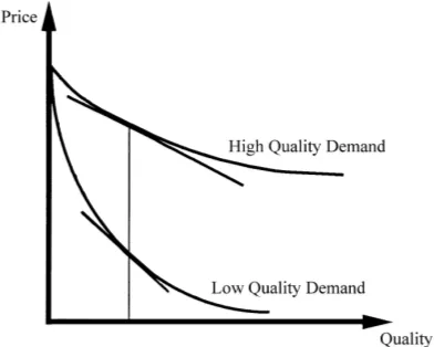
Fig. 1. Demands that imply introductory pricing under private information: the higher inverse demand is flatter and both demands are weakly convex.
The first sentence of the proposition simply requires that second period demand be an increasing function of the belief that quality is high. The inequality in the second sentence contains two terms. The second term,−E[uXXX]/E[uXX], is the Arrow–Pratt measure of
the convexity of the inverse demand function in consumption (note that the inverse demand function isE[uX]). The numerator of the first term is the difference in slopes of the high
quality and low quality inverse demands. So this inequality is satisfied if both inverse demands are convex in quantity and the higher inverse demand is flatter than the lower, as in Fig. 1. A comparison with Mirman et al. (1993) is illuminating. They find that the firm sets a lower (mean) first period price if the higher inverse demand is flatter than the lower. Our model agrees with theirs that the firm does not experiment if the two inverse demands are parallel and linear. They do not require any convexity assumptions, but our proposition permits the slope condition to fail provided that demand is sufficiently convex (as in our Examples 2 and 3). Of course the rationale for introductory pricing is quite different in their model. In their model the firm experiments to affect its own learning and information is always valuable to it; the issue is to determine when higher output is more informative. In our model the firm uses the price to affect consumer learning and higher consumption is more informative by assumption; the issue is to determine when information is valuable to the firm. The next three examples verify that some frequently used specifications satisfy the condi-tions in Theorem 2: quadratic utility, implying linear (interior) demands; constant elasticity demands; and semi-log demands. In each case the second period equilibrium price is inde-pendent of first period consumption, allowing for some heterogeneity in buyer preferences.
Example 1(Linear demands). Let buyern’s utility be given byun(X, θ )=αX−Bn(θ )
(12)X2, whereα > 0 andBn(.) is a positive, decreasing function of θ. Let En[Bn] =
ρnBn(θH)+(1−ρn)Bn(θL). The second period demand isDn(P , ρn) = max{0, (α−
P )/En[Bn]}, which is strictly convex inρn for interior choices. Note moreover that the
of buyers, and hence of first period consumption. Thus each buyer’s first period demand correspondence will be decreasing in the first period price, and the firm will engage in introductory pricing.
Example 1 is consistent with Mirman et al. (1993): for two linear demand curves with the higher inverse demand flatter than the lower, the firm prices lower initially.
Example 2 (Constant elasticity demands). un(X, θ ) = (βn/α)(θ X)α with 0 < α <
1, and βn > 0 Buyer n’s demand is Dn(P , ρn) = P(α−1)
−1
Bn(ρn), whereBn(ρn) =
(αnEn[θα])(1−α)
−1
. This demand is strictly convex inρn. Aggregate demand isP(α−1)
−1 B, whereBis the sum of theBnterms of buyers. Again the equilibrium second period price
is independent of beliefs and hence of period 1 consumption. Thus if buyers all have pref-erences of this form, the firm will charge an introductory price.
The demands in Example 3 would lead tolowerfirst period output, and hence higher mean period 1 price, in Mirman, Samuelson and Urbano, since the higher inverse demand is steeper than the lower. The next example would lead to neither lower nor higher first period outputs in their model, though it does lead to introductory pricing in ours.
Example 3(Semi-log demands). Letun(X, θ )=An(θ )X+βR0Xln(ω)dω, whereAn(.)
is a positive, increasing function ofθ, andβ >0. The demand for buyernisDn(P , ρn)=
exp{(En[An(θ )]−P )/β}, and the aggregate demand isBexp{−P /β}, whereBis the sum
of the exp{En[An(θ )]/β}, terms across buyers. Again each buyer’s demand is convex in
beliefs and the second period price is independent of beliefs.
5. Concluding remarks
In a two-period model in which both buyers and the seller are uncertain about product quality, but in which buyers may experiment to gain more information, we have given sufficient conditions for first period price to be lower than what would maximize first period profit, our definition of an introductory price. We presented two versions of the model: identical buyers with a public quality signal (Theorem 1) and heterogeneous buyers with private consumption signals (Theorem 2).
For the representative buyer case we showed that quasilinear utility was sufficient for introductory pricing. For the case of different buyers and private quality signals we identified a subset of quasilinear preferences that lead to introductory pricing; a sufficient condition is that the inverse demands are convex and the higher inverse demand is flatter than the lower. The subset includes linear, constant elasticity and semi-log demands.
Acknowledgements
I thank Hector Chade, Tony Creane, Drew Fudenberg, Bruno Jullien, Dave Mandy, Len Mirman, Mike Ormiston, Harris Schlesinger and seminar participants in Toulouse, Lund and the Southeastern Economic Theory meetings at SMU for discussions and comments on drafts of this paper. An anonymous referee of this journal and Associate Editor John Conlisk also made several useful suggestions. Part of this research was done while visiting IDEI at the University of Toulouse and I am grateful to that institute for its support. This work was funded in part by a grant from the Arizona State University College of Business.
Appendix A
We use the following definition in some of our proofs.
Definition 5(Milgrom and Shannon, 1994). LetXbe a subset ofRnandT a subset ofR
and leth(.)be a real-valued function onX×T.h(.)satisfies the single crossing property in(x, t ) if forx′ > x′, andt′ > t, h(x′, t ) > h(x, t ) impliesh(x′, t′) > h(x, t′)and
h(x′, t )≥h(x, t )impliesh(x′, t′)≥h(x, t′).
Proof of Proposition 1. Suppose that the information structure satisfy (S1). We need to show thatω(x) = RF (ρ(z, x))f (z, x)dzis increasing inxfor any convex continuous functionF (.), wheref (z, x)=ρ0g(z−ψ(x, θH))+(1−ρ0)g(z−ψ(x, θL)). It follows
readily thatω(.)is increasing for any convex continuous functionF (.)if it is increasing for any continuously differentiable convex functionF (.). Differentiating with respect tox
yields23
Following the argument in Section VII (up to Eq. 28) of Mirman et al. (1994), we may, after integrating by parts twice, writeω′(x)as
ω′(x)= −(ψx(x, θH)−ψx(x, θL))(1−ρ0)
Thus, integrating by parts we get that
ω′(x)=(ψx(x, θH)−ψx(x, θL))(1−ρ0)
Z
ρ(z, x)g(z−ψ(θL, x))d[F′(ρ(z, x))]≥0.
Proof of Proposition 2. For part (i) let (x0,−p0) ∈ e−(0), (x∗,−p∗) ∈ e−(1). We must show that(x0,−p0)∧(x∗,−p∗) ∈ e−(0)and(x0,−p0)∨(x∗,−p∗) ∈ e−(1). For the “inf” part, if(x0,−p0)∧(x∗,−p∗) = (x0,−p0), we are done. If p∗ > p0,
then x∗ ≤ x0, sinced(., ρ0)is decreasing. So (x0,−p0)∧ (x∗,−p∗) = (x∗,−p∗). Nowp∗x∗−c(x∗)+δWs(x∗) ≥ p0x0−c(x0)+δWs(x0), p0x0−c(x0) ≥ p∗x∗− c(x∗), andWs(x∗)≤ Ws(x0)sop0x0−c(x0)=p∗x∗−c(x∗)and hence(x∗,−p∗) ∈ e−(0). Ifx∗ < x0, then we again havep0x0−c(x0) =p∗x∗−c(x∗). Sinced(.ρ0)is decreasing,p∗≥p0, so(x0,−p0)∧(x∗,−p∗)=(x∗,−p∗)∈e−(0). For the “sup” part, if(x0,−p0)∨(x∗,−p∗) =(x∗,−p∗), we are done. Ifp0 < p∗, thenx∗ ≤ x0. Hence
Ws(x∗)≤Ws(x0), which together withp0x0−c(x0)≥p∗x∗−c(x∗)implies that the “sup” (x0,−p0)∈e−(1). Ifx∗< x0, thenWs(x∗)≤Ws(x0). Moreoverp∗≤p0sinced(.ρ0)
is decreasing. Thus the “sup”(x0,−p0)∈e−(1), which proves part (i). To prove part (ii), suppose thatWs(.)is strictly increasing on an interval containing 0 and{x|(x, p)∈e(0)},
but thate−(1)≥Ce−(0)fails. Then there exists a(x0,−p0)∈e−(0), (x∗,−p∗)∈e−(1)
with eitherx∗ < x0orp∗ > p0. Ifx∗ < x0then we havep∗x∗−c(x∗)+δWs(x∗) ≥ p0x0−c(x0)+δWs(x0)andp0x0−c(x0)≥p∗x∗−c(x∗). These inequalities together
imply thatWs(x∗)≥Ws(x0), contradicting the assumption thatWs(.)is strictly increasing
on an interval containing [0, x0]. Ifp∗ > p0, then sinced(.;ρ0)is decreasing, we must havex∗≤x0. A strict inequality is ruled out by the foregoing argument. Ifx∗ =x0, then that contradicts(x0,−p0)∈e−(0):p0x0−c(x0) < p∗x∗−c(x∗). This establishes part (ii). Part (iii) follows from standard comparative statics arguments.
Proof of Theorem 2. The proof follows from arguments used to establish Theorem 1.
Proof of Proposition 5. Convexity of demand follows by implicitly differentiating the first order condition for the buyer’s problem,p=E[uX], twice with respect toρ. The remaining
part of the theorem lists various sufficient conditions for the first period demand for each buyer to be decreasing in the first period price,p. (i) is trivial. For (ii), suppose thatp′′> p′
but thatd(p¯ ′, P′′) >d(p¯ ′, P′), where the second argument is the second period equilibrium price associated with the corresponding first period price, and all other arguments of the de-mands are suppressed. By hypothesis,P′′≥P′, since all buyers have identical preferences. IfP′′=P′, then we get a contradiction: the objective function for the first period demand correspondence given in Definition 3 is supermodular in(xn,−p), implying it is decreasing
inpfor a fixedP. IfP′′> P′, then observe first thatd(p¯ ′′, P′)≤ ¯d(p′, P′)by the preced-ing argument. Next we show thatWb(.)is supermodular in(xn,−P ). We have∂Wbn/∂P =
−R
D(P , ρ(zn, xn))f (zn, xn)dzn, after applying the envelop theorem. Since demand is
convex in beliefs, and higher consumption is more informative, increases inxn increase
expected demand. ThusWb(.)is supermodular in(xn,−P ), implying that each buyern’s
first period objective is supermodular in(xn,−P )and hence thatd(p¯ ′′, P′′)≤ ¯d(p′′, P′).
Henced(p¯ ′′, P′′) ≤ ¯d(p′′, P′) ≤ ¯d(p′, P′), contradictingd(p¯ ′′, P′′) > d(p¯ ′, P′). The
References
Aghion, P., Espinosa, M., Jullien, B., 1993. Dynamic duopoly with learning through market experimentation. Economic Theory 3, 517–540.
Bagwell, K., Riordan, M., 1991. High and declining prices signal product quality. American Economic Review 81, 224–239.
Bergemann, D., Valimaki, J., 1996a. Learning and strategic pricing. Econometrica 64, 1125–1150.
Bergemann, D., Valimaki, J., 1996b. Market experimentation and pricing. Cowles Foundation Discussion Paper No. 1122.
Blackwell, D., 1951. Comparison of experiments. In: Neyman, J. (Ed.), Proceedings of the Second Berkeley Symposium on Mathematical Statistics and Probability. University of California Press, Berkeley, CA. Creane, A., 1994. Experimentation with heteroskadastic noise. Economic Theory 4, 275–286. Cremer, J., 1984. On the economics of repeat buying. RAND Journal of Economics 15, 396–403.
Cyert, R.M., Degroot, M.H., 1980. Learning applied to utility functions. In: Arnold, Z. (Ed.), Bayesian Analysis in Econometrics and Statistics. North-Holland, Amsterdam, pp. 159–168.
Grossman, S., Kihlstrom, R., Mirman, L.J., 1977. A Bayesian approach to the production of information and learning by doing. Review of Economic Studies 44, 533–547.
Harrington, J., 1995. Experimentation and learning in a differentiated products duopoly. Journal of Economic Theory 66, 275–288.
Judd, K., Riordan, M., 1994. Price and quality in a new product monopoly. Review of Economic Studies 61, 773–789.
Kihlstrom, R., 1984. A Bayesian exposition of Blackwell’s theorem on the comparison of experiments. In: Marcel, B., Richard, K. (Eds.), Bayesian Models in Economic Theory. North-Holland, Amsterdam, pp. 13–32. Lazear, E., 1986. Retail prices and clearance sales. American Economic Review 76, 14–32.
McFadden, D.L., Train, K.E., 1996. Consumers’ evaluation of new products: learning from self and others. Journal of Political Economy 104, 683–703.
Milgrom, P., Roberts, J., 1986. Price and advertising signals of product quality. Journal of Political Economy 94, 96–821.
Milgrom, P., Shannon, C., 1994. Monotone comparative statics. Econometrica 62, 157–180.
Mirman, L.J., Samuelson, L., Urbano, A., 1993. Monopoly experimentation. International Economic Review 34, 549–564.
Mirman, L.J., Samuelson, L., Schlee, E.E., 1994. Strategic information manipulation in duopolies. Journal of Economic Theory 62, 363–384.
Radner, R., Stiglitz, J.E., 1984. A nonconcavity in the value of information. In: Marcel, B., Richard, K. (Eds.), Bayesian Models in Economic Theory. North-Holland, Amsterdam, pp. 33–52.
Rockafeller, R.T., 1970. Convex Analysis. Princeton University Press, Princeton, NJ.
Schlee, E.E., 1996a. The value of information about product quality. RAND Journal of Economics 27, 803–815. Schlee, E.E., 1996b. Learning about product quality and introductory pricing. mimeo.
Shannon, C., 1995. Weak and strong monotone comparative statics. Economic Theory 5, 209–227. Shapiro, C., 1983. Optimal pricing of experience goods. Bell Journal of Economics 14, 497–507.