Directory UMM :Data Elmu:jurnal:M:Multinational Financial Management:

(1)

Journal of Multinational Financial Management 10 (2000) 345 – 365

A study of cointegration and variance

decomposition among national equity indices

before and during the period of the Asian

financial crisis

Hsiao-Ching Sheng

a

_{, Anthony H. Tu}

b,

_*

a_{Taiwan Power Company}_,_Taipei_, _Taiwan_,_ROC

b_{Department of Finance}_,_{College of Commerce}_,_{National Chengchi Uni}₆_ersity_,_Taipei_11623, _Taiwan_, ROC

Received 15 July 1999; accepted 27 March 2000

Abstract

This study uses a cointegration and variance decomposition analysis to examine the linkages among the stock markets of 12 Asia – Pacific countries, before and during the period of the Asian financial crisis. Johansen (1988) multivariate cointegration and error-correction tests demonstrate evidence in support of the existence of cointegration relationships among the national stock indices during, but not before, the period of financial crises. In the recent crisis, the relationship within the South-East Asian countries seems to be stronger than that within the North-East Asian countries. The variance decomposition reveals that the ‘degree of exogeneity’ for all indices has been reduced, implying that no countries are ‘exogenous’ to the financial crisis. In addition, Granger’s causality test suggests that the US market still ‘causes’ some Asian countries during the period of crisis, reflecting the US market’s persisting dominant role. © 2000 Elsevier Science B.V. All rights reserved.

JEL classification:C1; C3; F3

Keywords:Asian financial crisis; Cointegration; Variance decomposition

www.elsevier.com/locate/econbase

* Corresponding author. Tel.: +886-2-29387423; fax:+886-2-29393394.

E-mail address:g7357015@grad.cc.nccu.edu.tw (A.H. Tu).

(2)

H.-C.Sheng,A.H.Tu/J.of Multi.Fin.Manag.10 (2000) 345 – 365 346

1. Introduction

The economic and financial turmoil that struck Asia in mid 1997 was representa-tive of both crisis and panic. Asia’s financial systems had continued to rely upon what Professor Merton Miller has called ‘19th century technology’. Capital markets were poorly developed and, on the upside of the business cycle, banks extended credit excessively, misallocated capital and employed weak credit controls. When the Thailand Baht was devalued on July 2, 1997, panic spread among both foreign and domestic creditors and investors. In the following months, this was transmitted to other Asian Countries. Eventually, a group of countries (Thailand, Korea, Indonesia, Malaysia, Japan and the Philippines) suffered severe collapse of curren-cies and stock markets. Other countries (China, India, Hong Kong, Taiwan and Singapore) have, so far, suffered only the indirect consequences of the crisis.

Earlier evidence was provided by Malliaris and Urrutia (1992) that informational linkage among national capital markets is a factor responsible for financial crisis. They detected the causal relationships among national stock markets during the October 1987 stock market crash, finding a dramatic increase in bi-directional and uni-directional causality during the month of the crash. In contrast, no lead-lag relationships were detected for the periods before and after the crash. Eun and Shim (1989) empirical results also indicate that there exists a substantial degree of interdependence among national stock indices. Unexpected movements in interna-tional stock markets seem to have become influential news event that affect domestic stock markets. King and Wadhwani (1990) investigated why, in October 1987, almost all the stock markets fell together despite widely differing economic circumstances. They examined a rational expectations price equilibrium and mod-eled ‘contagion effects’ between markets. They found that an increase in volatility in one market, leads in turn to an increase in the size of the contagion ellects on other markets. They claim that their theory can provide a partial of explanation why the world stock markets uniformly fell during the October 1987 crash. Hamao et al. (1990) examined the prices and price volatility spillover effect among New York, London and Tokyo markets using an ARCH-type model. Evidence of price volatility spillovers from New York to Tokyo, London to Tokyo and New York to London was observed, bot no price volatility spillover effects in other directions were apparent for the pre-October 1987 period.

Recently, financial market liberalization and rapid development of telecommuni-cations networks has increased significantly the ability to transmit and disseminate information between markets. Bekaert and Harvey (1997) found that capital market liberalization did increase the correlation between local market returns and the world market, but did not drive up local market volatility. Also, Longin and Solnik (1995) found an upward trend in international correlations over the past 30 years, particularly in the rise of the correlations in periods of high volatility.

(3)

and Ho (1991) and Cheung (1993) examined the correlation structure among eleven emerging Asian stock markets and developed markets. They concluded that the correlation between the emerging Asian stock markets group and the developed market group was smaller than among the developed markets. However, based on various analytical techniques, the correlation matrix is not stable over time. Using cointegration analysis, Corhay et al. (1993) also investigated the price indices of five European stock markets and found that they displayed a common long-run trending behavior over the period 1975 – 1991. Choudhry (1997) investigated the long-run relationship between the stock indices of six Latin American countries and the United States, and found evidence of cointegration and significant causality among the six Latin American indices with and without the United States index. Christofi and Pericli (1999) explored the short-run dynamics between five major Latin American stock markets. They modeled the joint distribution of stock returns using a vector autoregression model with errors following a multivariate exponen-tial GARCH process and found evidence of first and second moment interactions among these markets.

The purpose of this paper is to analyze the linkages among national stock markets before and during the period of the Asian financial crisis. It is well known that the linkages among stock markets vary over time, and we examine whether there exist different degrees of linkages before and during the period of the Asian financial crisis. In contrast to the procedure used by Engle and Granger (1987) in Malliaris and Urrutia (1992), we employed Johansen (1988) multivariate cointegra-tion and errorcorreccointegra-tion model to investigate the nature and extent to which national stock markets contribute to the crisis process1_{. Moreover, we decompose}

the forecast error variance to show the proportion of the movements in one market due to its own shocks versus shocks from other markets. This can help us to understand how markets are ‘fully exogenous’ to the financial crisis, and whether the ‘degree of exogeneity’ differs before and during the period of the financial crisis. The multivariate cointegration and error-correction tests provide some evidence to support the existence of cointegrational relationships among the national stock indices during, but not before, the period of the financial crisis. The relationship in the South-East Asian countries seems to be stronger than that in the North-East Asian countries. The forecast error variance decomposition demonstrates that the ‘degree of exogeneity’ for all indices has been reduced, implying that no countries are ‘exogenous’ to the financial crisis. In addition, Granger’s causality test suggests that the US market still ‘causes’ all the Asian countries during the period of crisis, reflecting the US market’s persisting dominant role.

The paper is organized as follows: Section 2 describes the data. Section 3 presents the test of unit root, cointegration and error correction, causality and their results.

1_{Although Engle and Granger (1987)provide the cornerstone research linking cointegrated series that}

(4)

Section 4 introduces the forecast error variance decomposition model and its result. Section 5 summarizes and concludes the paper.

2. Data description

The data consist of daily closing prices for the New York S&P 500 index and the following 11 major Asia – Pacific equity market indices: Tokyo Nikkei 225, Hong Kong Hang-Seng, Singapore Straits Times, Sydney All Ordinaries, Seoul Com-posite Index, Taiwan ComCom-posite Index, Kuala Lumpur ComCom-posite Index, Manila Composite Index, Bangkok Composite Index, Jakarta Composite Index and Shang-hai B-shares index. The prices are collected for the period from July 1, 1996 to June 30, 1998.

To investigate the possible differences of cointegrational relationship among the 12 stock market indices before and during the Asian crisis, the data are divided into two groups:

1. July 1, 1996 – June 30, 1997: the period before the crisis. 2. July 1, 1997 – June 30, 1998: the period during the crisis.

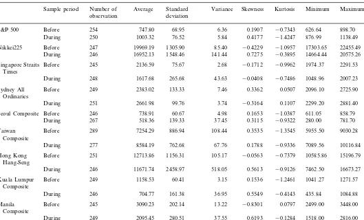
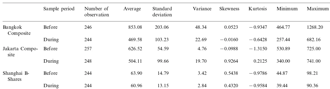
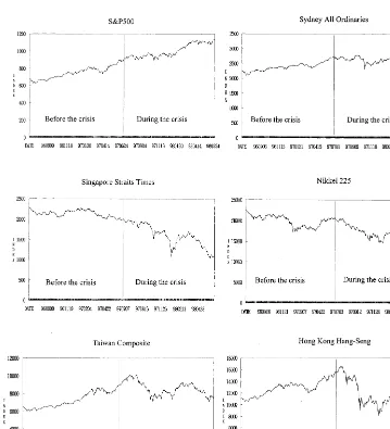
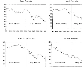
All daily index prices are taken a natural logarithm (ln) in front. Table 1 shows statistical characteristics in the 12 country indices. We also plot the 12 indices time series in Fig. 1 for the period before the crisis and for the period during the crisis. In order to ensure the same number of observations, we omitted all the observa-tions from Saturday’s trading (mainly in Bangkok, Taiwan and Seoul). For a specific (not common) holiday in a country, we use the preceding day’s observation as a proxy for that day.

3. Unit roots test

Following the discussion by Dickey and Fuller (1979, 1981), consider the time series of (xt) has thepth-order autoregressive process:

xt=a0+a1xt-1+a2xt-2+...+apxt−p+ot (1)

The representation can be transformed and added by a time-trend term.

Dxt=a0+rxt−1+a2t+ %

In the above Augmented Dickey – Fuller test, the null hypothesis is H0: r=0. If

this is true, xt has a unit root. Dickey and Fuller (1979) found that the critical

(5)

H

Statistical characteristics of the 12 countries’ indices

Number of Standard

Sample period Average Variance Skewness Kurtosis Minimum Maximum

observation deviation

0.1907

S&P 500 Before 254 747.80 68.95 6.36 −0.7343 626.64 898.70

0.4177 −1.4247 876.99 1138.49 5.84

250

During 1003.32 76.52

Before 247 19969.19 85.40 −0.4229 −1.0957 17303.65 22455.49

Nikkei225 1305.90

1548.46 141.44 0.7275 −0.3895 14664.44 20575.26

246 16952.13

During

2.68 −0.1712 −0.9962 1974.37

2136.59 2291.53

Singapore Straits Before 245 75.67

Times

During 248 1617.68 265.68 43.63 −0.0408 −0.7486 1048.96 2007.23

Before 249 133.33 7.46 0.3362 0.0507 2096.10 2725.90

Sydney All 2383.02

Ordinaries

−0.3164 0.1107 2299.20 2881.40

99.76 3.74

2661.98 251

During

60.67 4.98 0.1653 −1.0387 611.05 858.79 246

Seoul Composite Before 738.91

0.3115 −0.9322 280.00 781.70 37.45

518.36 267

During 139.33

886.94

Before 289 7254.29 108.44 0.3535 −1.3545 5955.50 9030.28

Taiwan Composite

0.1788 −0.9336 7089.56 10116.84

During 277 8584.19 762.68 67.76

105.17 −0.0563 −0.7379 10585.86

12713.86 15196.79

Hong Kong Before 251 1156.31

Hang-Seng

During 246 11671.74 2458.97 518.05 0.5613 −0.9126 7462.50 16673.27 3.15 0.1536 −1.2461 1041.27 1271.57 60.41

Before 249 1158.53

Kuala Lumpur Composite

36.95

During 246 704.77 161.38 0.5549 −0.4143 435.84 1084.88

202.14

Before 245 3090.23 13.22 −0.8301 0.0797 2499.00 3448.00

Manila Composite

0.6193 −0.1284 1518.00 2816.00 280.51

(6)

H

Sample period Average Variance Skewness Kurtosis Minimum Maximum

observation deviation

853.08 203.06 48.34 0.0523 −0.9347 464.77 1268.20

Bangkok Before 246

Composite

−0.0160 −0.6428 257.44 682.16 103.23 22.69

469.58 244

During

Before 257 54.59 4.76 −0.0988 −1.3150 530.89 725.00

Jakarta Compo- 626.52

site

0.9264 0.2125 340.00 741.00 99.66

During 248 504.11 19.70

3.42 0.5438 −0.9786 44.87

Shanghai B- Before 244 63.90 14.79 98.21

Shares

0.4320 −0.9584 39.44 90.36 13.15

(7)

t. Including an intercept term but not a trend term (a2=0 only), use the section

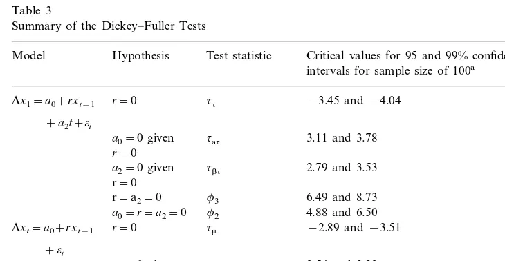
labeled tm. Finally, with both intercept and trend, use the section labeledtt., Table 2 lists critical values for 95 and 99% confidence intervals for t-statistict,tmandtt. Dickey and Fuller (1981) provided three additionalF-statistics (f1,f2andf3) to

test joint hypothesis on the coefficients. The null hypothesis r=a0=0 is tested

using the f1 statistic. Including a time trend in the regression, the joint hypothesis

a0=r=a2=0 is tested using the f2, statistic and the joint hypothesisr=a2=0 is

tested using the f3 statistic. Table 3 also provides critical values for 95 and 99%

confidence intervals for t-statisticf1, f2 and f3.

(8)

Fig. 1. (Continued)

Finally, it is possible to test hypotheses concerning the significance of the drift terma0and time trenda2. Under the null hypothesisr=0, the test for the presence

of the time trend is given by the tbt statistic. Thus, the statistic is the test a2=0

given thatr=0. Similarly, to test the hypothesisa0=0 given thatr=0 use thetat

(9)

H

.-C

.

Sheng

,

A

.

H

.

Tu

/

J

.

of

Multi

.

Fin

.

Manag

.

10

(2000)

345

–

365

353

Table 2

Summary results of unit roots testsa

South Korea

US Japan Singapore Australia Taiwan Hong Kong Malaysia The Philippines Thailand Indonesia China

Country

I(1)

I(1) I(1) I(1) I(1) I(1) I(1) I(1) I(1) I(0) I(1) I(1)

Before the crisis

I(1) I(1) I(1) I(1) I(1) I(1) I(1)

I(1)

During the crisis I(1) I(1) I(1) I(1)

(10)

values of 95 and 99% confidence intervals fortbt,tatandtamare also listed in Table 3.

Unless the researcher knows the actual data-generating process, it is questionable as to whether it is appropriate to estimate. Hence, we consider the following three alternatives of Eq. (2).

It might seem reasonable to test the hypothesis r=0 using the most general of the models of Eq. (2). For example, if the true process is a random walk, this regression should find that a0=r=a2=0. One problem with this line of reasoning

is that the presence of the redundant estimated parameters reduces degrees of freedom and the power of the test. In other words, there is the possibility that the research will conclude that the process contains a unit root, where, in fact, none is present.

Campbell and Perron (1991) found four important difficulties concerning the unit root tests. These difficulties imply that the research may fail to reject the null hypothesis of a unit root because of a mis-specification concerning the deterministic part of the regression. Too few or too many regressors may cause a failure of the

Table 3

Summary of the Dickey–Fuller Tests

Test statistic

Hypothesis Critical values for 95 and 99% confidence Model

intervals for sample size of 100a tt

(11)

test to reject the null of a unit root2_{. To avoid the inappropriate use of a unit root}

test, we follow the procedure suggested by Doldado et al. (1990).

The empirical results of unit root tests are summarized in Table 2. Before the crisis, the calculated values of test statistics, with the exception of Thailand, are all smaller than their corresponding critical values at 5% significance level. We do not reject the null hypothesis that the 11 indices (not Thailand) contain a unit root. During the period of the crisis, the calculated values of test statistics of all 12 indices are smaller than their corresponding critical values at 5% significance level. We do not reject the null hypothesis that the 12 indices all contain a unit root.

4. Cointegration and causality

4.1. Tests for cointegration and error-correction

Malliaris and Urrutia (1992) used the two-step procedure of Engle and Granger (1987) (EG hereafter) to test the cointegrational relationships among price move-ments on six different markets during the market crash of October 1987. EG’s procedure has been shown to be most appropriate for systems of only two variables with one possible cointegrating vector. Recent advances in multivariate cointegra-tion and error correccointegra-tion modeling provide a useful framework for analyzing equilibrium price adjustments in information-linked markets. Johansen (1988) and Stock and Watson (1988) maximum likelihood estimators can circumvent the use of EG’s two-step estimators and estimate and test for the presence of multiple cointegrating vectors. Moreover, these tests allow the researchers to test restricted versions of the cointegrating vectors and the speed of adjustment parameters.

Following Johansen (1988) procedure, we focus on the model3

Xt=A0+A1Xt−1+ot (3)

This can be rewritten as

DXt=A0+PXt−1+ot P=A1−I (4)

Both procedures by Johansen (1988) and Stock and Watson (1988) rely heavily on the relationship between the rank of P and its characteristic roots. The key feature to note in Eq. (4) is the rank of the matrix P; the rank of P equals the number of cointegrating vectors. Clearly, if rank (P)=0, the matrix is null. Since there is no linear combination of the (xit) processes that is stationary, the variables

are not cointegrated. Instead, if Pis of rankn, the vector process is stationary. In intermediate cases, if rank (P)=1, there is a single cointegrating vector and

2_{For details concerning the difficulties of the unit root tests refer to Campbell and Perron (1991) or}

Enders (1995).

3_{We follow Sims (1980) procedure and find that the optimal lag length is 1. Alternatively, you may}

(12)

expressionPXt−1 is the error correction factor. For other cases in which 1Brank

(P)Bn, which are multiple cointegrating vectors.

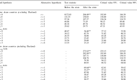
We first examine the cointegrational relationship among nine Asian countries (excluding Thailand due to its stationary properties): Japan, Singapore, South Korea, Taiwan, Hong Kong, Malaysia, the Philippines, Indonesia and Mainland China. The results are presented in Table 4. At 95% confidence interval, ltraceand

lmaxtests both show there is one cointegrating vector during the period of the crisis,

but none before the period of the crisis. Including Thailand, we then re-examine the cointegrational relationship among ten Asian countries. Table 4 also summaries the results. It shows that there are two cointegrating vectors during the period of the crisis, representing the key role of Thailand in the Asian financial crisis. Since Thailand’s index isI(0), we ignore only examination of the cointegrational relation-ship before the period of the crisis.

In the aftermatch of the crisis, we found that the cointegrational relationship had improved in the Asian countries as a whole. It is interesting to further examine the cointegrational relationship in each economic or political region in Asia. In the following empirical tests, we divide the 12 country indices into two groups:

North-East Asia group: Japan, South Korea, Taiwan, Hong Kong and China. South-East Asia group: Thailand, Malaysia, the Philippines, Singapore and Indonesia4_.

4.2. Granger’s causality

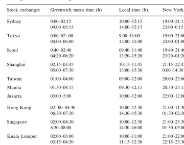
As found in Eun and Shim (1989), the US stock market is the most influential in the world. Shocks in the US stock market are rapidly transmitted to other markets in clearly recognizable movements. In this section, we employ Granger’s (1969) causality methodology to see whether the lead – lag relationship between the U.S. and Asian stock markets differs before and during the period of the financial crisis. Due to the fact that national equity markets are generally operating time zones with different opening and closing times, testing for lead – lag (or causality) relation-ships between US and Asian markets presents a problem of data synchronization due to time-zone shift differences. The adjustment of the causality test is of primary importance in the execution and interpretation of the empirical tests conducted in this study. Table 5 shows the trading hours of the national stock exchanges in Greenwich mean time, local time, and New York time. The middle column (local time) of Table 5 shows that all of the 11 Asia – Australia stock exchanges in our sample trade within or around the same time interval. Further, all of the Asia – Aus-tralia exchanges are closed when the New York Stock Exchange (NYSE) opens for the day. The last column (New York time) of Table 5 indicates that in any given trading day the closing prices for all of the Asia – Australia exchanges in our sample are already known by the time the NYSE closes for the day.

(13)

H

Test of cointegration among Asian countriesa

Critical value 90% Null hpothesis Alternative hypothesis Test statistic Critical value 95%

After the crisis Before the crisis

Nine Asian countries(excluding Thailand)

r\ 186.39

r=0 0172.03 204.49** 192.89

150.53

Ten Asian countries(including Thailand)

ltracetests

a_r_{denotes the number of cointegrating vectors. Critical values are summarized from Johansen and Juselius (1990).}

** and

(14)

Table 5

Trading hours of stock exchanges

New York time (h)

Hong Kong 02: 00–04:30 10:00–12:30 21:00–11:30 01:30–02:30

New York 1430–21:00 09:30–16:00 09:30–16:00

Following Malliaris and Urrutia (1992), we make the following adjustments for the Granger causality. Suppose that a major world event occurs in Hong Kong (or other exchange in Asia) and is announced at a certain point in time on a given trading day. The closing price of the same trading day on the S&P 500 index in New York will reflect this information. This illustrates that closing prices on dayt in Hong Kong (or other exchange in Asia) affect closing prices in New York on the same calendar day t. Thus, a Granger regression investigating whether Hong Kong (or other exchange in Asia) leads New York looks as follows:

Xt

(15)

Xt+1

HK

=g0+%

P

i=1

aiXt−i US

+ %

P

j=1

bjXt−j HK

+ot

4.3. Results

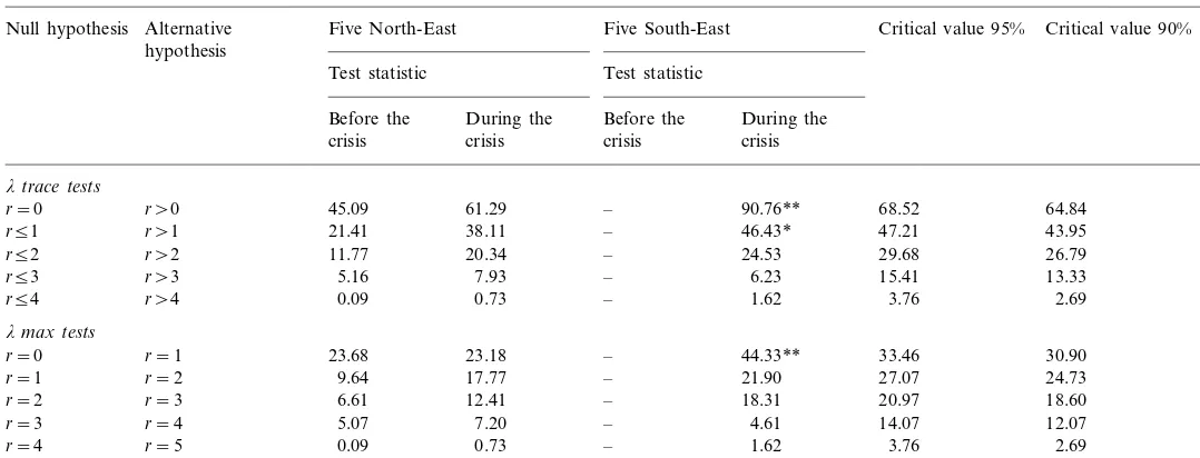
The results of cointegration tests for each group are given in Table 6, which shows that there is no evidence of any cointegrational relationship for the five North-East Asian country indices during (and before) the period of the crisis. However, the evidence shows that at least one cointegrational relationship exists for the five South-East Asian country indices during the period of the crisis.

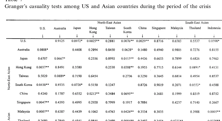
The results of the Granger’s causality tests are presented in Table 7. Each entry in the table denotes the P-value of the market on the left-hand side caused by the market at the top. The dominant role of the US stock market remains unchanged during the whole period of the financial crisis, and the results in Table 7 indicate that the US market still causes some Asian markets during the period of the financial crisis. Behind South Korea, the US market plays the second dominant role in the Asian financial crisis. On the other hand, only three Asian markets (Hong Kong, South Korea and China) cause (feedback) the US market. According to the above results, the Asian financial crisis seems to have been not an intra-regional crisis affecting only the equity markets in East Asia.

Table 7

(16)

H

Test of cointegration among five North-East and five South-East Asian countriesa

Five South-East Critical value 95% Critical value 90% Alternative

a_r_{denotes the number of cointegrating vectors. Critical values are summarized from Johansen and Juselius (1990).}

** and

(17)

H.-C.Sheng,A.H.Tu/J.of Multi.Fin.Manag.10 (2000) 345 – 365 361 5. Variance decomposition

As we know, a vector autoregression (VAR) can be written as a vector moving average (VMA). Thus, Eq. (3) can be iterated backward infinite times to obtain

X=m+_%

j=0

A1jot−j (5)

where m=(I+A1+A2+…)A0 is the unconditional mean of Xt.

The fact that Eq. (5) is the VMA representation of Eq. (3) in that variables (xit)

are expressed in terms of the current and past values of the various types of shocks (oit). The VMA representation of Eq. (3) is an essential feature of Sims (1980)

methodology in that it allows a tracing out of the time path of the various shocks on the variables contained in the VAR system. Since there are 11 variables (excluding Thailand) in our system, there will be totally 11×11=121 impulse response functions. It is extremely complicated to plot the impulse response functions to represent the behavior of the (Xit) series in response to the various

shocks (eit).

Instead, we choose to use ‘forecast error variance decomposition’ to show the proportion of the movements in a sequence (say country 1, x1t) due to its own

shocks (oit) versus shocks from other countries (e2t–o11t). If we use Eq. (5) to

conditionally forecast Xt+n the n-period forecast error is

Xt+n−EtXt+n= %

n−1

j=0

A1jot+n−j

Focusing solely on thex1t, sequence, we see that the variance of then-step ahead

forecast error variance of x1t+n is

s1(n)

represents the proportion of movements in country 1, x1t, due to shocks from

country i, oit.

Ifo2t, –o11tshocks explain none of the forecast error variance ofx1tat all forecast

horizons, we can say that the xlt, sequence is ‘fully exogenous’. In such a

circumstance, the x1t sequence would evolve independently of the o2t–o11t, and x2t–x11t, sequence. At the other extreme, o2t–e11t shocks could explain all the

forecast error variance in the x1t sequence at all forecast horizons, so that x1t

sequence would be ‘fully endogenous’. The ratio Wi(i), fori=1, 2,…11 that is the

(18)

Table 8

Variance decomposition (before the crisis)

ait, can be used to represent the ‘degree of exogeneity’ of country i in response to the financial crisis. We also compare the ratio for each country before and during the period of the crisis, in order to understand whether the ‘degree of exogeneity’ was reduced as a response to the financial crisis.

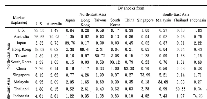
Tables 8 and 9 present, respectively, the results of variance decomposition for the period before, and during, the crisis. Each entry in the tables denotes the percentage of forecast error variance of markets on the left-hand side explained by the markets at the top. These entries are all convergent values in 24-day horizon. To facilitate the understanding of Tables 8 and 9, we also plot the results in Fig. 2.

Table 10 shows the proportion of market movements that can be explained by its own shocks, or the ‘degree of exogeneity’, before and during the period of the crisis. This indicates that the ‘degree of exogeneity’ for all countries has been significantly reduced, implying no countries are exogenous to the financial crisis. The degree of exogeneity in three markets, US, Australia and Taiwan, was reduced less (7.68, 4.00 and 7.67%, respectively). This also suggests that the markets of Australia and Taiwan passively responded to other country’s innovations during the period of the Asian financial crisis.

6. Summary

(19)

(20)

among the national stock indices during the period of the financial crisis. The relationship for the South-East Asian countries was stronger than that for the North-East Asian countries. The tests also show no cointegrational relationship before the period of the financial crisis. The forecast error variance decomposition also finds that the degree of exogeneity for all countries indices has been reduced,

Table 9

Variance decomposition (during the crisis

Table 10

The comparison of ‘degree of exogeneity’ before and during the period of the crisis Degree of exogeneity (%)

Before the crisis (1) During the crisis (2) Difference (1)−(2) 93.50

United States (US) 85.82 7.68

17.36 52.69

Japan (JA) 70.05

89.76 85.76

Australia (AU) 4.00

69.41 12.30

Hong Kong (HK) 57.11

72.32 17.40

Malaysia (MA) 89.72

Taiwan (TA) 93.12 85.45 7.67

29.18 93.38

Singapore (SI) 64.20

73.99 44.05

South Korea (SK) 29.94

15.68

84.09 68.41

Mainland China (MC)

65.86 23.69

Thailand (TH) 89.55

74.23 13.97

Indonesia (IN) 60.26

24.48 54.72

(21)

implying that no countries are ‘exogenous’ to the financial crisis. In addition, Granger’s causality test suggests that the US market still causes some Asian countries during the period of crisis, reflecting the US market’s persisting dominant role.

References

Bekaert, G., Harvey, C.R., 1997. Emerging equity market volatility. J. Financ. Econom. 43, 29 – 77. Campbell, J.Y., Perron. R., 1991. Pitfalls and opportunities: what macroeconomists should know about

unit roots], Technical Working Paper 100, NBER Working Paper Series.

Cheung, Y.L., 1993. A note on the stability of the interternporal relationships between the Asian – Pacific equity markets and the developed markets-a non-parametric approach. J. Bus. Financ. Account. 20, 223last-page\229.

Cheung, Y.W., Ho, L.K., 1991. The intertemporal stability of the relationship between the Asian emerging equity markets and the developed equity markets. J. Bus. Financ. Account. 18, 235 – 254. Choudhry, I., 1997. Stochastic trends in stock prices:evidence from Latin American markets. J.

Macroeconom. 19, 285 – 304.

Christofi, A., Pericli, A., 1999. Correlation in price changes and volatility of major Latin American stock markets. J. Multinat. Financ. Manage. 9, 79 – 93.

Corhay, A., Tourani Rad, A., Urbain, J.P., 1993. Common stochastic trends in European stock markets. Econom. Lett. 42, 385 – 390.

Dickey, D., Fuller, W.A., 1979. Distribution of the estimates for autoregressive time series with a unit root. J. Am. Stat. Ass. 74, 427 – 431.

Dickey, D., Fuller, W.A., 1981. Likelihood ratio statistics for autoregressive time series with a unit root. Econometrica 49, 1057 – 1072.

Divecha, A.B., Drach, I., Stefec, D., 1992. Emerging markets:a quantitative perspective. J. Portfolio Manage. 19, 41 – 45.

Doldado, I., Jenkinson, T., Sosvilla-Rivero, S., 1990. Cointegration and unit roots. J. Econom. Surveys 4, 249 – 273.

Enders, W., 1995. Applied Econometric Time Series. Wiley, New York.

Engle, R.E., Granger, C.W.J., 1987. Cointegration and error-corretion: representation, estimation, and testing. Econometrica 55, 251 – 276.

Eun, C.S., Shim, S., 1989. International transmission of stock market movements. J. Financ. Quantit. Anal. 24, 241 – 256.

Hamao, Y., Masulis, R.W., Ng, V., 1990. Correlation in price changes and volatility across international stock markets. Rev. Financ. Studies 3, 281 – 307.

Johansen, S., 1988. Statistical analysis of cointegration vectors. J. Econom. Dynam. Control 12, 231 – 254.

Johansen, S., Juselius, K., 1990. Maximum likelihood estimation and inference on cointegration with application to the demand for money. Oxford Bull. Econom. Stat. 52, 169209.

King, A.M., Wadhwani, S., 1990. Transmission of volatility between stock markets. Rev. Financ. Studies 3, 5 – 33.

Longin, E., Solnik, B., 1995. Is the correlation in international equity returns constant: 1960 – 1990? J. Int. Money Finance 14, 26.

Malliaris, A.G., Urrutia, J.L., 1992. The international crash of October 1987: causality tests. J. Financ. Quant. Anal. 27, 353 – 364.

Sims, C., 1980. Macroeconomics and reality. Econometrica 48, 149.

Stock, L., Watson, M., 1988. Testing for common trends. J. Am. Stat. Ass. 83, 1097 – 1107.