University of Bonn, Germany
[email protected], [email protected]
KEY WORDS:object categorization, facade image interpretation, bag of words
ABSTRACT:
Our objective is the categorization of the most dominant objects in facade images, like windows, entrances and balconies. In order to execute an image interpretation of complex scenes we need an interaction between low level bottom-up feature detection and high-level inference from top-down. A top-down approach would use results of a bottom-up detection step as evidence for some high-high-level inference of scene interpretation. We present a statistically founded object categorization procedure that is suited for bottom-up object detection. Instead of choosing a bag of features in advance and learning models based on these features, it is more natural to learn which features best describe the target object classes. Therefore we learn increasingly complex aggregates of line junctions in image sections from man-made scenes. We present a method for the classification of image sections by using the histogram of diverse types of line aggregates.
1 INTRODUCTION
Our objective is the interpretation of facade images that leads to a detailed description including dominant objects such as windows, entrances and balconies. Image interpretation of complex scenes in general needs an interplay between some high-level model for the co-occurrence of these objects and some low-level model for the appearance of these objects. This paper focuses on the catego-rization of objects in a facade, which is meant to serve a top-down module as a link to the image data. The scope of the paper is to classify subsections of images based on the histogram of relevant aggregates of straight line segments in a bag of words approach. To motivate the idea of learning a feature representation for fa-cade objects we will give a brief synopsis of recent work in the field of facade image interpretation.
We divide recent approaches into several fields of interests. The first group deals with the task of window detection from single images. There are two main approaches, either using gradient projection to find aligned edges (Lee and Nevatia, 2004; Recky and Leberl, 2010) or using a classificator that detects regions of interest by searching over the image (Ali et al., 2007; Jahangiri and Petrou, 2009). The first approach is restricted to facade types of which windows fulfil the alignment assumption, while the sec-ond approach does not take any alignment or structure assump-tion respectively into account. The work of Tylecek and Sara (2010) is an exception. Their work can be seen in between win-dow detection and exploiting repetitive structure. They propose a complex generative model in which they include object geometry as well as neighbourhood relations.
The next group of works performs a pixel wise labelling or facade segmentation. One powerful direction is the combination of a strong pixel wise classification like Random Forests (RF) with an unsupervised segmentation (Fr¨ohlich et al., 2010). Teboul et al. (2010) formulate a constrained generic shape grammar to express special types of buildings. They train a RF classificator to deter-mine a relationship between semantic elements of the grammar and the observed image support. Thus, a pixel wise classification is used as low-level input for the grammar. Another interesting approach is the hierarchical segmentation proposed by Berg et al.
(2007). They first parse the image into a coarse set of classes which are further parsed into more detailed classes using meta knowledge from a coarse level of detail. Both are handled within an MRF framework. This can be directly transferred to rules of a grammar, although not done in this work.
We believe that explicit modelling dominant facade objects gives much better evidence to guide a top-down interpretation system. In contrast to these approaches which deal with pixel wise evi-dence to guide top-down methods, we propose to learn generic parts of facade objects to allow object categorization from object specific image sections1, not whole scenes yet, see Figure 1 for some examples of given data. Object detection is easily realized afterwards by constructing a sliding window over whole facade images.
Widely used object categorization methods either use a number of object specific features (Fergus et al., 2003) or they learn a huge codebook of local image patches (Leibe et al., 2004) which results in a huge search space for matching image features within this codebook. Recently there are new approaches that deal with learning the parts that represent individual object classes, (Amit et al., 2004; Fidler et al., 2006, 2009; Gangaputra and Geman, 2006), thus avoiding fixed and pre-selected features.
Inspired by ideas of Fidler et al. (2009) and guided by the special structure of facade objects we propose a bottom-up approach to learn generic parts of object structure from given training image sections of these facade objects. We learn increasingly complex aggregates of lines from image sections showing individual ob-jects of the target classes. Finally we use learned line aggregates to classify new unseen image segments of learned target classes using the histogram of diverse types of line aggregates.
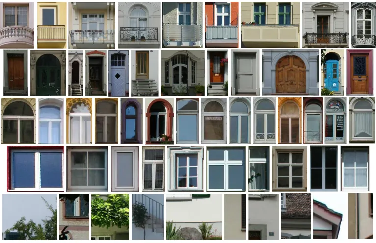
Figure 1: For each row some examples of given image sections for class balcony, entrance, arc-type windows, rectangular windows and background.
shows how to select the relevant aggregates. Section 3 explains our experiments and used data which are discussed in Section 3.2. We conclude with Section 4.
2 APPROACH
The basic idea of our approach is to classify rectified image sec-tions based on the histogram of relevant aggregated straight line segments.
2.1 Overview
Straight line segments reveal a large invariance to shadows and changes in illumination. Especially windows show a large variety in appearance, in particular due to the mirroring of other objects in the window panes, which let line segments appear as promising image features. Line aggregates show a large distinctiveness for certain object categories of facades, in case not only pairs of lines are taken into consideration. Therefore we use larger aggregates, say up to five lines, in order to arrive at rich image primitives. We allow aggregates to contain smaller ones as parts. Aggre-gates show typical configurations depending on the angles, see Figure 3. Not all aggregates are relevant for the classification. We therefore select those aggregates that help the classification. These learned aggregates show structures that are typical for cer-tain objects at facades, see Figure 4. We use the histograms of these relevant aggregates as features for classification. The com-plete approach is sketched in Figure 2, p. 3. We start from given training image sections, together with their labels, see top row of Figure 2. From these images we first collect all possible aggre-gatesA = {Ak}of lines. The aggregates are partitioned into subsetsAdof aggregates consisting ofdlines. Each aggregate Ak has a certain typetk ∈ T which is a function of the num-berdof lines and their directions, rounded to multiples ofπ/8. The setT of all possible types of aggregates can be seen as the language for describing our objects. Learning which types are relevant for describing the target classes results in the vocabu-laryV ={vi} ⊂ T. Classification is done by a simple bag of words (BoW) approach: we interpret identified aggregates of type
4 3
A
2
A
1
A
A
Figure 3: (Best viewed in colour) Toy example to visualize the meaning of aggregates of lines. We start from lines collected in the setA1. Aggregates of A2 are given by line junctions; each aggregate is shown in a different colour. Aggregates of
A3 are groups of three lines, thus elements ofA2 joining one line. They are visualized by twoA2aggregates joining the same colour. Overlapping aggregates are shown behind each other. Ag-gregatesA4with four lines are built accordingly to the previous lines, adding one line to all elements inA3. Thus they are junc-tions of four lines, visualized by threeA2aggregates joining the same colour.
vias words of a vocabularyV as it is usually done in BoW ap-proaches. Thus an image section is represented by the histogram
h(vi), vi∈ Vof aggregate types restricted to the learned vocabu-lary. Taking this as feature vectorx= [h(vi)]we train an import vector machine (IVM), as proposed by Roscher et al. (2012). This was shown to get a state of the art classification performance. It is a discriminative classifier, therefore usually ensures better dis-criminative power than generative models and it produces class wise probabilities for test samples.
Having learned the vocabularyV and the IVM model, we clas-sify a new image section (bottom row of Figure 2) by detecting aggregates of the vocabulary, taking its histogram and estimating its most probable class using the IVM model.
Next we describe how to build the aggregates. 2.2 Building the aggregates
V
{A | t }
for Testing
Image Training
i
[h(v )]
k kTest Label
Figure 2: The scheme: Starting from labelled training images, we derive a set{Ak}of aggregatesAkwith general typetk ∈ T for each image and select those aggregates that belong to relevant typestk∈ V. The vocabularyVhasIelements. We use the histogram h = [h(vi)]of the aggregates of each image as a feature vector for the supervised classification. Given a test image we derive the relevant features and use their histogram for deriving its label.
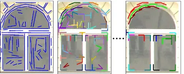
Figure 4: (Best viewed in colour) Detected aggregates from the learned set of relevant aggregate types for one given image sec-tion. Left: lines detected by FEX,A1. Middle: relevant line junctions,A2 aggregates. Right: relevant aggregates from five lines,A5aggregates. As aggregates are possibly mutual overlap-ping, not all junctions are visible.
from straight line-features together with their adjacency graph structure using FEX as described in F¨orstner (1994) and Fuchs and F¨orstner (1995). This is different to Fidler et al. (2006) and Fidler et al. (2009), in which they preferably use Gabor-wavelets as they try to model arbitrary object classes. The benefit of using the FEX-procedure is the additional information about the neigh-bourhood relations of pair wise lines without having to depend on their distance and size. Thus we become independent of a certain neighbourhood size. The neighbourhood of two lines is defined with the Voronoi-diagram of extracted lines. Those lines who join a Voronoi-edge are said to be neighboured.
All neighbouring lines are combined toA2 aggregates in case they are not parallel, thus building junctions which are the inter-section points of the lines. The junctions of two neighbouring lines have two typesτ of relation to the lines: Either the inter-section point is outside of a line, thenτ = 1, otherwiseτ = 2. An instance of anA2 aggregate is parametrized by its orienta-tionφ ∈ ]− 180◦. . . 180◦], thus the direction of the first
line, the angleα ∈ [0. . .180◦[between the two lines and the
types(τ1, τ2) ∈ [1,2]of their mutual connectivity. Please note that connectivity (middle-middle) is not allowed, as this would be a crossing that is no valid outcome from edge extraction. All angles are discretized inπ/8 = 22.5◦ steps, thus we have 16
bins for orientation and 8 bins for the angle. Together with three possible values for line connectivity, we have 384 different line junctions. Given these definitions we code the geometry ofA2 aggregates by unique numbers between 1 and 384, which define all possible types ofA2. Detected instances ofA2aggregates are
stored as a listA2 =
a2
k witha
2
k= (tk;xk)wheretk∈ T is
a type of the language andxkthe position in the image section. To get aggregates of the next level of complexity we sequentially add neighbouring lines to already existing aggregates. The typet
of aAdpart is coded by the type names of involvedA2parts and the angleωbetween the added line and the existing configura-tion, again discretized into 16 bins, which gives about 2 million possible configurations forA3parts, more than 14 billion forA4 etc.
Please note that there is neither a scale nor any other configuration details, except for directions, included. Due to a high variability of facade objects, the clustering of dominant distances between neighbouring line junctions fails. Thus, we ignore distances and just collect co-occurrences of line-junctions and cluster directions between them.
Next we describe how we learn the relevant aggregates. 2.3 Feature selection
In the beginning we just know the languageT =ti, thus all pos-sible aggregate types. Now we are looking for a subsetV ⊂ T
of relevant aggregates. The histograms using all types are of a very large dimension, usually contains many zeros and further-more not all types are relevant for the classification. We therefore identify those bins of the histogram that are informative in terms of classification, which is a typical feature selection problem. LetX be the set of all available featuresxi = h(ti), i.e. the number of occurring aggregates of typeti. The task of feature selection is to find a setS ⊂ X ofmfeaturesxi ∈ X which have the largest dependency on their individual target classc. As a measure for dependency, correlation and mutual information are widely used. It is known that feature sets chosen this way are likely to have high redundancy, thus the dependency between individual features is high, and they are therefore not informa-tive. Following this argumentation Peng and Ding (2005) pro-posed a feature selection algorithm called Max-Relevance Min-Redundancy (MRMR). To describe dependency between features or features and labels, they use mutual entropy which is given by the expectation of the mutual information and defined by
H(x;y) =−X
x
X
y
p(x, y) ln p(x, y)
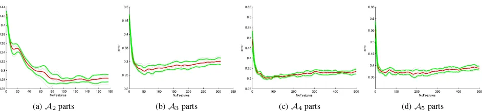
(a)A2parts (b)A3parts (c)A4parts (d)A5parts
Figure 5: Feature selection, error curves depending on the number of selected features. gray: classification error for different testsets, red: mean error, green:1σband.
for two random variablesxandy. The maximal dependency be-tween an individual featurexiand labelcis given by the largest mutual entropyH(xi;c). To select a setSˆrelof features with the
largest dependency on labelscone searches for features satisfy-ing the so-called Max-relevance condition.
ˆ
But for selecting mutual exclusive featuresSˆredone can use the
condition called Min-Redundancy
In both cases, solving the minimization and maximization prob-lem, respectively, is intractable due to the huge number of possi-ble combinations of features.
Therefore Peng and Ding (2005) propose an approximation by a sequential forward selection. Assume we already have a setSi,
initialized by using Equation 1, thus selecting the feature with the highest mutual entropy with its class label
S1 = arg max
x
H(x;c) (4)
In each step that feature is added, which maximizes the MRMR-criterion
Si+1=Si∪arg max xj∈X \Si
Q (5)
for which Peng and Ding (2005) propose to use either the differ-ence
forQ, between relevance and redundancy. In our experiments we tested both criteria and got slightly better results using (7). We use a Matlab implementation provided by Peng and Ding (2005) to successively select most relevant but less redundant parts. Thus, in the learning step, after collecting allAd parts
for each training image we perform MRMR feature selection to get thoseAdtypes that fulfil these requirements.
Unfortunately one needs to define the number of features to be selected before hand, which is one of the main unknown parts of our procedure, as we know neither types nor number of relevant features. We solve this by selecting a sufficiently large number
of parts by MRMR, which gives a ranking of best suited features and estimate the classification error depending on the number of features. Usually the classification error decreases while added features are still informative and stagnates or even increases. We therefore successively add one feature after the other and esti-mate the classification error using a simple k-nearest neighbour classifier with a five-fold cross validation on given training sam-ples. After smoothing we choose the number of features with the lowest estimated classification error. Figure 5 shows the average (red) classification error depending on the number of features for four different levels of complexity of the vocabulary.
3 EXPERIMENTS
3.1 Experimental setup
We choose a challenging dataset with five classes namely bal-conies, entrances, arc-type windows, rectangular windows plus background samples with 400, 76, 198, 400 and 400 samples per class, respectively, see Figure 1, p. 2 for some examples. For each sample image its target classcis given. These sam-ples are taken from annotated rectified facade images, such that each sample image contains exactly one object of its given target class. Background samples are sampled randomly from rectified facade images. Samples taken this way that accidentally con-tain too large parts of foreground objects are removed manually. Please note that they are not resized to have an equal size. The classification task is to learn a representation of this target class, in a way that we are able to classify new and unknown images to one of these classes.
We perform a five-fold cross validation. The dataset is equally split into five groups, such that different sample sizes per class are equally split, too. In each cross validation step we choose four of the groups for learning the relevant aggregates by using feature selection and the IVM model. The remaining group is used for testing, thus detecting proposed aggregates and testing the IVM model.
For learning we first collect all line pairs (junctions) for all im-ages from the learning set. Performing the feature selection over histograms from these aggregates define the vocabulary of aggre-gatesA2. For each following level of complexitydand again for every image section from the training set we further combine the already learned aggregates with new neighbouring lines. The fea-ture selection gives the set of learnedAdaggregates and therefore
(a)A2parts (b)A3parts (c)A4parts
Figure 6: Feature selection, examples for the first 49 selected parts ofA2toA4, extracted from one cross validation step. Please note that these results are similar in all cross validation steps.
words. Using the learned IVM model we got a prediction of the target class, which we compare to the given label to build the confusion matrix.
Next we show results of these experiments 3.2 Results and discussion
First we show some learned types of the vocabulary in Figure 6 forA2toA4.
Having the geometry of the target classes in mind this is a rea-sonable collection. ForA2we got rectangular junctions and ag-gregates that are suited to be part of an arc. AlsoA3 andA4 aggregates are reasonable parts of the target geometries. In
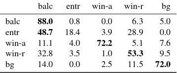
or-balc entr win-a win-r bg balc 88.0 0.8 0.0 6.3 5.0 entr 48.7 18.4 3.9 28.9 0.0 win-a 11.1 4.0 72.2 5.1 7.6 win-r 32.8 3.5 1.0 53.3 9.5 bg 14.0 0.0 2.5 11.5 72.0 Table 1: Confusion matrix in [%] for learning and testing just using aggregates ofA2, mean values from five-fold cross valida-tion, accuracy68.5. Lines: ground truth, rows: prediction, balc: balcony, entr: entrance, win-a: arc-type window, win-r: rectangular window
balc entr win-a win-r bg balc 85.3 2.3 1.0 7.0 4.5 entr 36.8 19.7 6.6 30.3 6.6 win-a 3.5 1.5 70.7 13.6 10.6 win-r 16.5 3.0 3.0 69.0 8.5
bg 8.8 1.0 2.0 4.2 84.0
Table 2: Confusion matrix just using aggregates ofA3, accuracy
75.2, see Table 1
der to test the classification performance we first use each subset
Adseparately. Results in terms of confusion matrices are shown
in Table 1 to 4. By just using line junction, aggregates ofA2give a reasonable classification performance. Balconies are classified with an88% true positive rate. Note that we are dealing with single images, thus we have no 3D information, which usually guides recognition of balconies. The confusion matrix proves that classification of entrances is a challenging task; they are mostly classified as balconies. The confusion between rectangu-lar and arc-type windows is low, which shows that just using line
balc entr win-a win-r bg balc 79.5 3.0 2.0 9.0 6.5 entr 25.0 22.4 9.2 38.2 5.3 win-a 3.0 2.5 69.2 12.6 12.6 win-r 9.0 3.8 4.5 74.5 8.2
bg 4.5 0.0 2.0 5.5 88.0
Table 3: Confusion matrix just using aggregates ofA4, accuracy
76.1, see Table 1
balc entr win-a win-r bg balc 80.0 3.0 1.3 10.0 5.8 entr 44.7 4.0 6.6 36.8 7.9 win-a 6.1 5.6 25.3 37.4 25.8 win-r 17.8 8.5 4.5 56.8 12.5
bg 6.0 0.5 2.5 6.5 84.5
Table 4: Confusion matrix just using aggregates ofA5, accuracy
63.6, see Table 1
junction, thus identifying rectangles and curves, generates good discriminative power for these classes. Using the other subsets separately for classification got slightly better results, exceptA5 where the classification performance significantly drops. Results
balc entr win-a win-r bg balc 92.3 1.0 0.3 2.0 4.5 entr 40.8 26.3 3.9 26.3 2.6 win-a 8.1 6.6 74.7 5.6 5.1 win-r 22.0 7.5 1.0 63.0 6.5
bg 10.0 1.3 2.5 8.5 77.8
Table 5: Confusion matrix using aggregates ofA2andA3, accu-racy74.6, see Table 1
for testing the classification performance using several subsets
Adare shown in Table 5 to 7. We see that using aggregates of
different complexity significantly increases the classification per-formance. Using aggregates fromA2up toA5gives an overall classification accuracy of almost80%. Please note that we cor-rectly identify balconies, rectangular and arc-type windows with
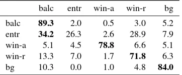
balc entr win-a win-r bg balc 89.3 2.0 0.5 3.0 5.2 entr 34.2 26.3 2.6 28.9 7.9 win-a 5.1 4.5 78.8 6.6 5.1 win-r 13.3 7.0 1.7 71.8 6.3
bg 10.3 0.0 1.0 4.8 84.0
Table 6: Confusion matrix using aggregates ofA2,A3andA4, accuracy78.4, see Table 1
balc entr win-a win-r bg balc 88.5 1.5 0.5 2.0 7.5 entr 28.9 34.2 3.9 23.7 9.2 win-a 4.0 3.5 81.3 4.5 6.6 win-r 9.8 8.5 1.3 73.8 6.8
bg 8.0 0.3 1.0 5.7 85.0
Table 7: Confusion matrix using aggregates ofA2toA5, accu-racy79.8, see Table 1
4 CONCLUSIONS AND FUTURE WORK
We proposed a method for classification using the histogram of types of relevant aggregates of straight line segments. For this we showed how to learn increasingly complex aggregates of line junctions from image sections from man-made scenes. Using these aggregates, provided a reasonable classification performance on a challenging dataset. For all we know, this is the first ap-proach of facade object categorization including balconies and entrances from single view images. The shown classification per-formance proves that the learned set of line aggregates is suited to give good evidence for existence of certain facade objects from bottom-up. This can be done when including the approach into an object detection method like sliding window or using it as a region classifier. This will be used in future work to guide a top down scene interpretation that will not be restricted to pixel wise evidence. Furthermore we will investigate how to include length information into the definition of aggregate types.
References
Ali, H., Seifert, C., Jindal, N., Paletta, L. and Paar, G., 2007. Win-dow detection in facades. In: Proc. of the 14th International Conference on Image Analysis and Processing, pp. 837–842. Amit, Y., Geman, D. and Fan, X., 2004. A coarse-to-fine strategy
for multi-class shape detection. Transactions on Pattern Anal-ysis and Machine Intelligence (PAMI) 28, pp. 1606–1621. Berg, A. C., Grabler, F. and Malik, J., 2007. Parsing images of
architectural scenes. In: Proc. of the International Conference on Computer Vision (ICCV), pp. 1–8.
Fergus, R., Perona, P. and Zisserman, A., 2003. Object class recognition by unsupervised scale-invariant learning. In: Proc. of the Conference on Computer Vision and Pattern Recogni-tion (CVPR), Vol. 2, pp. 264–271.
Fidler, S., Berginc, G. and Leonardis, A., 2006. Hierarchical sta-tistical learning of generic parts of object structure. In: Proc. of the Conference on Computer Vision and Pattern Recogni-tion (CVPR), Vol. 1, pp. 182–189.
Fidler, S., Boben, M. and Leonardis, A., 2009. Object Cate-gorization, Computer and Human Vision Perspectives. Cam-bridge University Press, chapter Learning Hierarchical Com-positional Representations of Object Structure, pp. 1–18.
F¨orstner, W., 1994. A framework for low-level feature extrac-tion. In: Proc. of the European Conference on Computer Vi-sion (ECCV), Vol. 801/1994, pp. 383–394.
Fr¨ohlich, B., Rodner, E. and Denzler, J., 2010. A fast approach for pixelwise labeling of facade images. In: Proc. of the Inter-national Conference on Pattern Recognition (ICPR), pp. 3029– 3032.
Fuchs, C. and F¨orstner, W., 1995. Polymorphic grouping for im-age segmentation. In: Proc. of the International Conference on Computer Vision (ICCV).
Gangaputra, S. and Geman, D., 2006. A design principle for coarse-to-fine classification. In: Proc. of the Conference on Computer Vision and Pattern Recognition (CVPR), Vol. 2, pp. 1877–1884.
Jahangiri, M. and Petrou, M., 2009. An attention model for ex-tracting regions that merit identification. In: Proc. of the Inter-national Conference on Image Processing (ICIP).
Lee, S. C. and Nevatia, R., 2004. Extraction and integration of window in a 3d building model from ground view images. In: Proc. of the Conference on Computer Vision and Pattern Recognition (CVPR), Vol. II, pp. 113–120.
Leibe, B., Leonardis, A. and Schiele, B., 2004. Combined object categorization and segmentation with an implicit shape model. In: Proc. of the Workshop on Statistical Learning in Computer Vision.
Peng, Hanchuanand Long, F. and Ding, C., 2005. Feature selec-tion based on mutual informaselec-tion: criteria of max-dependency, max-relevance and min-redundancy. Transactions on Pattern Analysis and Machine Intelligence (PAMI) 27(8), pp. 1226– 1238.
Recky, M. and Leberl, F., 2010. Windows detection using k-means in cie-lab color space. In: Proc. of the International Conference on Pattern Recognition (ICPR), pp. 356–359. Roscher, R., Waske, B. and F¨orstner, W., 2012. Incremental
Import Vector Machines for Classifying Hyperspectral Data. Transactions on Geoscience and Remote Sensing. accepted. Teboul, O., Simon, L., Koutsourakis, P. and Paragios, N., 2010.
Segmentation of building facades using procedural shape pri-ors. In: Proc. of the Conference on Computer Vision and Pat-tern Recognition (CVPR), pp. 3105–3112.