this PDF file EFFECT OF COST INCREMENT DISTRIBUTION PATTERNS ON THE PERFORMANCE OF JIT SUPPLY CHAIN | Bidiawati J.R | Jurnal Teknik Industri 1 PB

(1)

EFFECT OF COST INCREMENT DISTRIBUTION PATTERNS

ON THE PERFORMANCE OF JIT SUPPLY CHAIN

Ayu Bidiawati J.R1, Noor Ajian Mohd Lair2.

1) _{Faculty of Industrial Technology, Industrial Engineering Department, Universitas Bung Hatta}

Jl. Gajah Mada, Gunung Panggilun, Padang, Sumatera Barat Email: ayubidiawati@yahoo.com

2)

Faculty of Manufacturing Engineering, Kolej Universiti Teknikal Kebangsaan Malaysia Durian Tunggal, Melaka, Malaysia

Email: noorajian@kutkm.edu.my

ABSTRACT

Cost is an important consideration in supply chain (SC) optimisation. This is due to emphasis placed on cost reduction in order to optimise profit. Some researchers use cost as one of their performance measures and others propose ways of accurately calculating cost. As product moves across SC, the product cost also increases. This paper studied the effect of cost increment distribution patterns on the performance of a JIT Supply Chain. In particular, it is necessary to know if inventory allocation across SC needs to be modified to accommodate different cost increment distribution patterns. It was found that funnel is still the best card distribution pattern for JIT-SC regardless the cost increment distribution patterns used.

Keywords: supply chain management, cost increment distribution Patterns, JIT-hybrid supply chain.

1. INTRODUCTION

Similar to production floor, Supply Chain Management (SCM) places greater emphasised on profit optimisation. The usual way to optimise profit is by minimising total cost (Shapiro, 2001). Considering this, various researches in supply chain operation research integrate cost as one of their performance measures such as Gullu (1997), Sabri and Beamon (2000), Petrovic et al. (1998), Omar and Shaharoun (2000), Larson et al. (1999) and Van Der Vost et al. (2000), while Lin et al. (2001) propose ways of accurately calculating cost by implementing activity-based costing (ABC) in managing logistics. Lin et al. (2001) suggested that the cost should be assigned to the resources for each logistics activities. Aggregating the cost into departments or sections will not represent true cost occurred at the corresponding sections. They claim that using ABC may provide accurate output of optimisation. Ingene and Parry (2000) reviewed the literature, which led them to conclude that product price is similar for each player at every echelon in a supply chain. Price discrimination is infeasible due to administrative, bargaining and contract development costs.

(2)

2. THE SUPPLY CHAIN

A SC studied by Closs et al. (1998) is selected as the hypothetical SC for this research. The supply chain was selected because it fulfilled all four requirement of basic SC structure and had extensive input and output data. Mohd Lair et al. (2003) present model selection and building in detail. The SC selected consists of a supplier (S), a manufacturer (M), two distributors (D) and three retailers (R) as shown in Figure 1. There is unlimited supply of raw material at the supplier. Tables 1 through 3 provide additional information of the SC (Mohd Lair et al., 2003).

Figure 1. Supply chain layout (adapted from Closs et al.,1998)

Table 1. Cycle time (in days)

Parameter Mean Distribution

Processing time supplier 1.0 Normal (std dev. = 0.3)

Processing time manufacturer 0.08 Triangular(min=0.02, max=0.2) Processing time distributor 0.3 Triangular (min = 0.1, max=1.0) Processing time retailer 0.5 Triangular ( min =0.2, max = 2.0

All transit times 5.0 (std dev. = 5)

Total lead time 21.9

Table 2. Transportation schedule and truckload

Transporters Schedule Load

To supplier Once per week

To manufacturer Once per week To distributor Twice per week

To retailer Twice per week

Truck capacity 24 units partial loads allowed

Table 3. Customer arrival pattern distributions

Customer arrival (demand pattern) Distribution

Low variability of demand Uniform (0.8,1.2)

High variability of demand Uniform (0.2,1.8)

R1

R2

R3 D1

D2 M

S

Material Flow

(3)

3. MODELLING AND EXPERIMENTATION

A model was developed using WITNESS® simulation software. The benefits of simulation were recognised and documented by Chisman (1992), Law and Mc. Gomas (1994) and Witness user’s Manual – Release 7.0 (1995). The selection criteria of the simulation Software was discussed in Law (1990), i.e. animation, computing time, model building time, customer support, minimum programming, customised report etc. After considering the criteria mentioned in Law and Mc. Gomas (1994), WITNESS® simulation software fulfilled the requirements. WITNESS® simulation software would be employed as the modelling tool. The model JIT Supply Chain was presented by Mohd Lair et al. (2003). The models are used to find means of determining the parameters for each card distribution pattern and cost increment distribution pattern strategy investigated. The models serve as initial testbed to analyse and evaluate the performance of JIT Supply Chain.

Most input data was as given by Closs et al. (1998) and additional necessary data was set based on extensive preliminary experiments. Before determining the warm-up period, a preliminary run was conducted to check whether the values of input parameters would deliver the expected performance of JIT SC that closely resembled to the Closs experiment. The simulation models developed were then run. Output data were analysed. The program was easily debugged using stepwise approach, i.e. change a few elements, run the model, verify it and then proceed on making changes. Validation was conducted by comparing the findings concluded from the simulation run with findings given by Closs et al. (1998). Detail discussions on model validation were presented in Mohd Lair

et al. (2003).

The JIT-Hybrid model identified as the best JIT strategy in Mohd Lair et al. (2003) was used as the based for experimentation. Two parameters involved in this experiment were card distribution patterns and cost increment distribution patterns. The card distribution patterns referred to bowl, inverted bowl, funnel, reversed funnel and uniform. Figure 2 illustrated the distribution patterns. Both cards and cost increment patterns were arranged according to the illustrated patterns.

In order to simplify study on four echelons SC, 20 cost objects with the smallest cost of 0.1 and biggest cost of 2.0 were selected. These values were selected as they can be distributed easily among the four echelons. Andijani (1997) provided formulas to calculate the total number of feasible allocation sets for the cost,

1

Using Formula 1, the feasible cost allocation sets for 4 echelons and 20 costs objects were:

(4)

The identified feasible cost allocation sets were then grouped into six groups; five groups each representing one of the five cost increment distribution patterns and a group of allocation sets that did not belong to any of the distribution patterns. Based on this, there was one allocation set for uniform, 63 sets for funnel and reversed funnel, 264 sets for bowl and 236 sets for inverted bowl. The remaining 342 allocation sets were unidentified. The identified and grouped allocation sets represented the five cost increment distribution patterns.

a) Uniform distribution pattern

b) Bowl distribution pattern

c) Funnel distribution pattern

d) Reverse funnel distribution pattern

e) Inverted bowl distribution pattern

(5)

The cost increment distribution patterns were then implemented on the models along with the corresponding card distribution patterns. The models are then modified to simulate different cost increment distribution patterns. The experiments on the models are conducted and analysed. The simulation results show the next section in detail.

4. RESULTS

Table 4 presents the means and ANOVA results comparing each card distribution pattern under cost increment distribution pattern. Based on the results presented, it is concluded that funnel card distribution pattern produced significant different for lowest inventory cost and bowl card distribution pattern produced significant different highest for total inventory cost.

Table 4. Comparing the means of total system inventory cost for bowl cost increment distribution pattern under five card distribution patterns

Total system inventory cost

Card pattern Mean (std. dev) Mean diff. (lowest) a Mean diff. (highest) b Bowl 126.73 (13.806) -10.156* -

Inverted bowl 122.54 (14.182) -5.972* 4.184* Funnel 116.57 (13.105) - 10.156*

Reversed funnel 123.46 (13.591) -6.886* 3.270* Uniform 122.48 (13.688) -5.906* 4.250*

• a

Comparing the lowest mean (row)against other means. Tested using ANOVA.

• b

Comparing the highest mean (row) against other means. Tested using ANOVA.

• * Indicates the mean difference is significant at α = 0.05.

• Shaded indicates pattern (row) with either the lowest or highest mean.

Table 5 presents the means and ANOVA results comparing each card distribution pattern under inverted bowl cost increment distribution pattern. Based on the results presented, it is concluded that funnel, inverted bowl, reversed funnel and uniform card distribution patterns produced significant lowest inventory cost and bowl, inverted bowl, reversed funnel and uniform produced significant highest total inventory cost.

Table 5. Comparing the means of total system inventory cost for inverted bowl cost increment distribution pattern under five card distribution patterns

Inverted bowl 120.37 (21.052) -4.636 2.822 Funnel 115.74 (19.813) - 7.458*

Reversed funnel 120.56 (20.848) -4.825 2.633 Uniform 120.09 (20.829) -4.348 3.110

• a

• b

• * Indicates the mean difference is significant at α = 0.05.

(6)

Table 6 presents the means and ANOVA results comparing each card distribution pattern under funnel cost increment distribution pattern. Based on the results presented, it is concluded that inverted bowl, funnel, reversed funnel and uniform card distribution patterns produced significant lowest inventory cost and bowl, inverted bowl, reversed funnel and uniform patterns produced significant highest total inventory cost.

Table 6. Comparing the means of total system inventory cost for funnel cost increment distribution pattern under five card distribution patterns

Inverted bowl 91.58 (11.49) -3.046 2.691 Funnel 88.27 (10.59) - 5.997*

Reversed funnel 92.32 (11.56) -4.046 1.951 Uniform 91.70 (11.44) -3.426 2.571

• a

• b

• * Indicates the mean difference is significant at α = 0.05

Table 7 presents the means and ANOVA results comparing each card distribution pattern under reversed funnel cost increment distribution pattern. Based on the results presented, it is concluded that funnel card distribution pattern produced significant lowest inventory cost and bowl, inverted bowl, reversed funnel and uniform patterns produced significant highest total inventory cost.

Table 7. Comparing the means of total system inventory cost for reversed funnel cost increment distribution pattern under five card distribution patterns

Inverted bowl 150.58 (10.60) -6.802* 3.802 Funnel 143.78 (10.22) - 10.604*

Reversed funnel 150.67 (10.38) -6.891* 3.713 Uniform 150.02 (10.47) -6.235* 4.369

• a

Comparing the lowest mean (row)against other means.

• d

Comparing the highest mean (row) against other means.

• Tested using ANOVA.

(7)

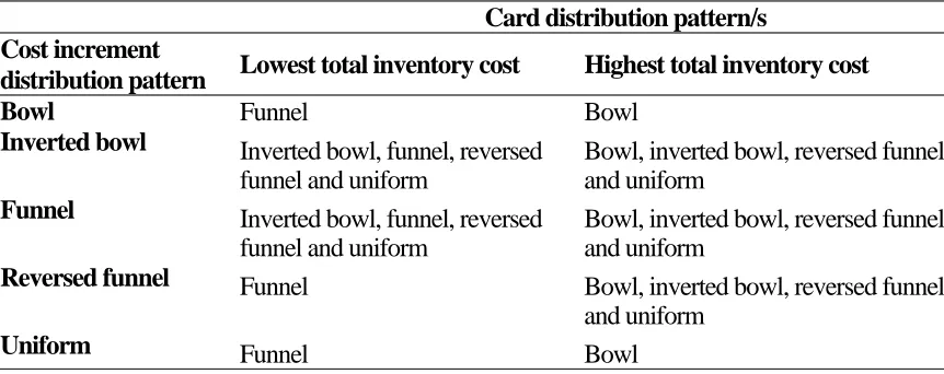
Table 9 summarizes all discussion above. The table shows that funnel card distribution pattern is still the best when various cost increment distribution patterns are applied. Moreover, arranging the card in bowl distribution pattern may cause the total system inventory cost to be higher than necessary, as more inventories are needed to operate this system.

Table 8. Comparing the means of total system inventory cost for uniform cost increment distribution pattern under five card distribution patterns

Inverted bowl 121.52 (0.47) -5.312* 3.509* Funnel 116.20 (0.84) - 8.821*

Reversed funnel 122.07 (0.72) -5.866* 2.954* Uniform 121.34 (0.63) -5.135* 3.686* • a

Comparing the lowest mean (row)against other means. Tested using ANOVA

• d

Comparing the highest mean (row) against other means. Tested using ANOVA

Table 9. Card distribution patterns representing the lowest and highest system inventory cost for each cost increment distribution pattern

Card distribution pattern/s Cost increment

distribution pattern Lowest total inventory cost Highest total inventory cost

Bowl Funnel Bowl

Inverted bowl _{Inverted bowl, funnel, reversed}

funnel and uniform

Bowl, inverted bowl, reversed funnel and uniform

Funnel _{Inverted bowl, funnel, reversed}

funnel and uniform

Bowl, inverted bowl, reversed funnel and uniform

Reversed funnel _Funnel _{Bowl, inverted bowl, reversed funnel}

and uniform

Uniform _{Funnel Bowl}

5. CONCLUSION

(8)

Therefore, the current practice of using units of inventory as performance measure is without regard to the cost increments along the JIT supply chain is justified. Recommendation for future work is to modify the generic models developed in this study and investigate other specific objectives and also expand the model of the actual system.

REFERENCES

Andijani, A., 1997. “Trade-Off between Maximizing Throughput Rate and Minimizing System Time in Kanban System.” International Journal of Operations &

Purchasing Management, Vol. 17, No. 5, p. 429−445.

Chisman, J.A., 1992. Introduction to Simulation Modeling Using GPSS/PC, Prentice-Hall, New Jersey.

Closs, D.J., Roath, A.S., Goldsby, T.J., Eckert, J.A., and Swartz, S.M., 1998. “An Empirical Comparison of Anticipatory and Response Based Supply Chain Strategies.” The International Journal of Logistics Management, Vol. 9, No. 2, p. 21−33.

Gullu, R., 1997. “A Two-Echelon Allocation Model and the Value of Information under Correlated Forecasts and Demands.” European Journal of Operation Research, Vol. 99, p. 386−400.

Ingene, C.A., and Parry, M.E., 2000. “Is Channel Coordination All It Is Cracked Up To Be?” Journal of Retailing, Vol. 76, No. 4, p. 511−547.

Larson, P.D., and DeMarais, R.A., 1999. “Psychic Stock: An Independent Variable Category of Inventory.” International Journal of Physical Distribution and

Logistics Management, Vol. 29, No. 7/8, p. 495–507.

Law, A.M., and Mc. Gomas, M.G., 1994. “Simulation Software for Communications Networks: The State of Art.” IEEE Communication Magazine, Vol. 3, p. 44−50.

Law, A.M., 1990. “Selecting Simulation Software.” Automation News, Vol. 5, No. 1, p. 3−8.

Lin, B., Collins, J., and Su, R.K., 2001. “Supply Chain Costing and Activity-Based Perspective.” International Journal of Physical Distribution & Logistics

Management, Vol. 31, No. 10, p. 702−713.

Mohd Lair, N.A, Nabi Baksh, Mohamed Shariff and Shaharoun, A.M., 2003. “A Comparison of JIT with Conventional Inventory Strategies in a Supply Chain.”

Proceedings of the 19thInternational Conference on CAD/CAM, Robotics and Factory of the Future, Kuala Lumpur, Malaysia July 22-24, p. 779−785.

Omar, M.K., and Shaharoun, A.M., 2000. “Coordination of Production and Distribution Planning in the Supply Chain Management.” Proceedings of the Second

International Conference on Advance Manufacturing Technology: ICAMT -2000,

Johor Bahru, Malaysia, p. 545–549.

(9)

Sabri, E.H., and Beamon, B.M., 2000. “A Multi Objective Approach to Simultaneous Strategic and Operational Planning in Supply Chain Design.” Omega, Vol. 28, p. 581−598.

Shapiro, J.F., 2001. Modeling the Supply Chain, Duxbury, Australia.

Van der Vost, J.G.A.J., Beulens, A.J.M., and Van Beek, P., 2000. “Modeling and Simulating Multi-Echelon Food Systems.” European Journal of Operational