https://dx.doi.org/10.24001/ijaems.3.3.5 ISSN: 2454-1311
Impact of Variable Ordering Cost and
Promotional Effort Cost in Deteriorated Economic
Order Quantity (EOQ) Model
Padmabati Gahan, Monalisha Pattnaik*
Dept. of Business Administration, Sambalpur University, Jyotivihar, Burla, India
Abstract— The instantaneous economic order quantity (EOQ) profit optimization model for deteriorating items is introduced for analyzing the impact of variable ordering cost and promotional effort cost for leveraging profit margins in finite planning horizons. The objective of this model is to maximize the net profit so as to determine the order quantity and promotional effort factor. For any given number of replenishment cycles the existence of a unique optimal replenishment schedule are proved and further the concavity of the net profit function of the inventory system in the number of replenishments is established. The numerical analysis shows that an appropriate policy can benefit the retailer, especially for deteriorating items. Finally, sensitivity analyses with respect to the major parameters are also studied to draw managerial decisions in production systems.
Keywords— Variable ordering cost, Promotional effort cost, Deterioration, Profit.
I. INTRODUCTION
Most of the literature on inventory control and production planning has dealt with the assumption that the demand for a product will continue infinitely in the future either in a deterministic or in a stochastic fashion. This assumption does not always hold true. Inventory management plays a crucial role in businesses since it can help companies reach the goal of ensuring prompt delivery, avoiding shortages, helping sales at competitive prices and so forth. The mathematical modeling of real-world inventory problems necessitates the simplification of assumptions to make the mathematics flexible. However, excessive simplification of assumptions results in mathematical models that do not represent the inventory situation to be analyzed.
Many models have been proposed to deal with a variety of inventory problems. The classical analysis of inventory control considers three costs for holding inventories. These costs are the procurement cost, carrying cost and shortage cost. The classical analysis builds a model of an inventory
system and calculates the EOQ which minimize these three costs so that their sum is satisfying minimization criterion. One of the unrealistic assumptions is that items stocked preserve their physical characteristics during their stay in inventory. Items in stock are subject to many possible risks, e.g. damage, spoilage, dryness; vaporization etc., those results decrease of usefulness of the original one and a cost is incurred to account for such risks.
https://dx.doi.org/10.24001/ijaems.3.3.5 ISSN: 2454-1311
Chaudhuri (1995) considered an economic order quantity (EOQ) inventory model for deteriorating goods developed with a linear, positive trend in demand allowing inventory shortages and backlogging. Bose, Goswami and Chaudhuri (1995) and Hariga (1996) investigated the effects of inflation and the time-value of money with the assumption of two inflation rates rather than one, i.e. the internal (company) inflation rate and the external (general economy) inflation rate. Hariga (1994) argued that the analysis of Bose, Goswami and Chaudhuri (1995) contained mathematical errors for which he proposed the correct theory for the problem supplied with numerical examples. Pattnaik (2011) explained a single item EOQ model with demand dependent unit cost and variable setup cost. Padmanabhan and Vrat (1995) presented an EOQ inventory model for perishable items with a stock dependent selling rate. They assumed that the selling rate is a function of the current inventory level and the rate of deterioration is taken to be constant. Pattnaik (2012) explained a non-linear profit-maximization entropic order quantity model for deteriorating items with stock dependent demand rate. Pattnaik (2013) introduced a fuzzy EOQ model with demand dependent unit cost and varied setup cost under limited storage capacity.
The most recent work found in the literature is that of Hariga (1995) who extended his earlier work by assuming a time-varying demand over a finite planning horizon. Pattnaik (2011) assumes instant deterioration of perishable items with constant demand where discounts are allowed. Pattnaik (2010) presented an entropic order quantity (EnOQ) model under instant deterioration for perishable items with constant demand where discounts are allowed. Salameh, Jabar and Nouehed (1999) studied an EOQ inventory model in which it assumes that the percentage of on-hand inventory wasted due to deterioration is a key feature of the inventory conditions which govern the item stocked.
Pattnaik (2011) discussed an entropic order quantity (EnOQ) model under cash discounts. Pattnaik (2012) introduced an EOQ model for perishable items with constant demand and instant deterioration. Pattnaik (2012) studied the effect of promotion in fuzzy optimal replenishment model with units lost due to deterioration. Pattnaik (2013) investigated linear programming problems in fuzzy environment with evaluating the post optimal
analyses. Pattnaik (2013) discussed wasting of percentage on-hand inventory of an instantaneous economic order quantity model due to deterioration. Raafat (1991) explained survey of literature on continuously deteriorating inventory models. Roy and Maiti (1997) presented fuzzy EOQ model with demand dependent unit cost under limited storage capacity. Tripathy, Pattnaik and Tripathy (2012) introduced optimal EOQ model for Deteriorating Items with Promotional Effort Cost. Tripathy, Pattnaik and Tripathy (2013) presented a decision-making framework for a single item EOQ model with two constraints. Tsao and Sheen (2008) explored dynamic pricing, promotion and replenishment policies for a deteriorating item under permissible delay in payment. Waters (1994) and Pattnaik (2012) defined various inventory models with managerial decisions. Wee (1993) explained an economic production lot size model for deteriorating items with partial back-ordering. In this model, replenishment decision under none wasting the percentage of on-hand inventory due to deterioration are adjusted arbitrarily upward or downward for profit maximization model in response to the change in market demand within the finite planning horizon with dynamic setup cost with promotional effort cost. The objective of this model is to determine optimal replenishment quantities and optimal promotional effort factor in an instantaneous replenishment profit maximization model.
https://dx.doi.org/10.24001/ijaems.3.3.5 ISSN: 2454-1311 development of the model. The mathematical formulation is developed in Section 3. The solution procedure is given in Section 4. In Section 5, numerical example is presented to illustrate the development of the model. The sensitivity analysis is carried out in Section 6 to observe the changes in the optimal solution. Finally Section 7 deals with the
α Percentage of on-hand inventory that is lost due to deterioration,
q Order quantity,
� × �− Ordering cost per cycle where, < � <
,
q* Traditional economic ordering quantity (EOQ),
(t) On-hand inventory level at time t,
Denote (t) as the on-hand inventory level at time t. During a change in time from point t to t+dt, where t + dt > t, the It is a differential equation, solution is
t =− ρα + q + αρ × e−αt
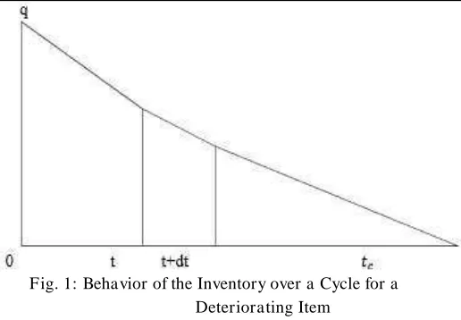
Where q is the order quantity which is instantaneously replenished at the beginning of each cycle of length tc units of time. The stock is replenished by q units
each time these units are totally depleted as a result of outside demand and deterioration. Behavior of the inventory level for the above model is illustrated in Fig. 1. The cycle length, tc, is determined by first substituting tc into equation
t and then setting it equal to zero to get: t =
αln
https://dx.doi.org/10.24001/ijaems.3.3.5 ISSN: 2454-1311
Fig. 1: Behavior of the Inventory over a Cycle for a Deteriorating Item
Equation t and � are used to develop the mathematical
model. It is worthy to mention that as α approaches to zero, � approaches to . The total cost per cycle, TC (q, ), is
The total profit per cycle with α approaching to zero only is
1(q,). 1(q,) = q× � – TC (q,) = � − � �− − −
In order to show the uniqueness of the solution in, it is sufficient to show that the net profit function throughout the cycle is jointly concave in terms of ordering quantity q and promotional effort factor . The second cycle with respect to q can be expressed as:
https://dx.doi.org/10.24001/ijaems.3.3.5 ISSN: 2454-1311
separately are strictly negative. The next step is to check that the determinant of the Hessian matrix is positive, i.e.
� ,
The objective is to determine the optimal values of q and to maximize the net profit function. It is very difficult to derive the optimal values of q and , hence unit profit function. There are several methods to cope with constraints optimization problem numerically. But here LINGO 13.0 software is used to derive the optimal values of the decision variables.
V. NUMERICAL EXAMPLE
Consider an inventory situation where K is Rs. 200 per order, h is Rs. 5 per unit per unit of time, r is 1200 units per unit of time, c is Rs. 100 per unit, the selling price per unit Ps is Rs. 125, � is 0.5 and � is 0%, � = . and � =1.0.
The optimal solution that maximizes equation , and
∗∗ and ∗are determined by using LINGO 13.0 version
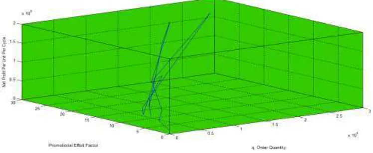
software and the results are tabulated in Table 2. In the present model the net profit, units lost due to deterioration, the cycle length and order quantity are comparatively more than that of the comparative models, it indicates the present model incorporated with promotional effort cost and variable ordering cost may draw the better decisions in managerial uncertain space. Fig. 2 represents the relationship between the order quantity q and dynamic setup cost OC. Fig. 3 represents the three dimensional mesh plot order quantity q, promotional effort factor and net profit per cycle . Fig. 4 is the sensitivity plotting of order quantity q, promotional effort factor and net profit per cycle , .
Table.2: Optimal Values of the Proposed Model
Model Iteration �∗ �∗ �∗ ∗ OC PE � � � behaviour. The computational results shown in Table 11.5.4 indicate the following managerial phenomena:
�the replenishment cycle length, q the optimal replenishment quantity, the optimal promotional effort factor, PE promotional effort cost, the optimal net profit per unit per cycle and the optimal average profit per unit per cycle are insensitive to the parameter K but OC variable setup cost is sensitive to the parameter K.
� the replenishment cycle length, q the optimal replenishment quantity, the optimal promotional effort factor, PE promotional effort cost, OC variable setup optimal replenishment quantity, PE promotional effort cost, the optimal net profit per unit per cycle and the
optimal average profit per unit per cycle are sensitive to the parameter r
�the replenishment cycle length, q the optimal replenishment quantity, the optimal promotional effort factor, PE promotional effort cost, OC variable setup cost, the optimal net profit per unit per cycle and the optimal average profit per unit per cycle are sensitive to the parameter c.
�the replenishment cycle length, q the optimal replenishment quantity, the optimal promotional effort factor, PE promotional effort cost, OC variable setup cost, the optimal net profit per unit per cycle and the optimal average profit per unit per cycle are sensitive to the parameter �.
�the replenishment cycle length and the optimal promotional effort factor, q the optimal replenishment quantity, PE promotional effort cost, the optimal net profit per unit per cycle and the optimal average profit per unit per cycle are insensitive to the parameter � and OC variable setup cost is sensitive to the parameter �.
https://dx.doi.org/10.24001/ijaems.3.3.5 ISSN: 2454-1311
q the optimal replenishment quantity, OC variable setup cost, PE promotional effort cost, the optimal net profit per unit per cycle and the optimal average profit per unit per cycle are sensitive to the parameter � .
�the replenishment cycle length is insensitive to the parameter � but the optimal promotional effort factor,
q the optimal replenishment quantity, OC variable setup cost, PE promotional effort cost, the optimal net profit per unit per cycle and the optimal average profit per unit per cycle are sensitive with static to the parameter
� .
Table.3: Sensitivity Analyses of the parameters K, h, r, c, � ,�,� �� �
Parameter Value Iteration �∗ �∗ ∗ OC PE � �, �,
K
150 83 5 99750.03 16.625 0.474934 585937.7 660937 132187.4 250 90 5.000001 99750.05 16.625 0.79155 585937.9 660936.7 132187.3 500 85 5.000001 99750.05 16.625 0.94987 585937.9 660936.6 132187.5 h
3 59 8.333334 270416.7 27.04167 0.3846 1627604 1752604 210312.4 8 120 3.125002 40371.15 10.76563 0.99539 228882.3 275755.8 88241.83 10 100 2.500002 26437.57 8.812515 1.23004 146484.9 183983.1 73593.19 r
1250 88 5.000001 103906.3 16.625 0.62045 610351.9 688475.9 137695.2 1300 80 5.000001 108062.5 16.625 0.60840 634765.9 716015.0 143203 1400 110 5.000001 116375 16.625 0.58627 683594 771093.2 154218.6 c
105 79 4.400001 69168.05 13.10001 0.76046 351384.4 409463.2 93059.8 108 81 4.000002 52800.06 11.00001 0.87039 240000.4 287999.1 71999.75 103 72 3.400003 33558.09 8.225014 1.09177 125282 159960.4 47047.13
�
120 76 4.000002 52800.06 11.00001 0.87039 240000.4 287999.1 71999.5 130 82 6 169200 23.5 0.48622 1215000 1323000 220499.9 132 86 6.4 204288 26.6 0.44250 1572864 1695744 264959.9
�
0.1 89 5 99750 16.625 0.00633 585937.5 660937.5 132187.5 0.3 72 5 99750.01 16.625 0.06336 585937.5 660937.4 132187.5 0.6 96 5.000002 99750.09 16.62501 2.00200 585938.3 660935.5 132187.1
�
3 76 5.000001 68500.04 11.41667 0.76416 890625.3 465624.2 93124.83 5 95 5.000002 43500.05 7.250006 0.95893 234375.4 309374 61874.78 10 103 5.000005 14750.06 4.125006 1.27128 117188 192186.2 38437.21
�
2 106 5.000042 6078.178 1.013021 2.56533 488.2977 75485.72 15097.02 3 92 5.000043 6000.117 1.000011 2.58196 0.4069150 74997.82 14999.44 4 85 5.000043 6000.052 1 2.58198 0.00339095 74997.42 14999.35
Fig.2: Two dimensional plot of Order Quantity, q and Dynamic Ordering Cost, OC
0 10 20 30 40 50 60 70 80 90 100
20 40 60 80 100 120 140 160 180 200
q, (Order Quantity)
O
C
,
(D
yn
am
ic
O
rd
er
in
g
C
os
t
pe
r
C
yc
le
https://dx.doi.org/10.24001/ijaems.3.3.5 ISSN: 2454-1311
Fig.3: Three Dimensional Mesh Plot of Order Quantity q, Promotional Effort Factor and Net Profit per Cycle ,
Fig. 4: Sensitivity Plotting of Order Quantity q, Promotional Effort Factor and Net Profit per Cycle ,
VII. CONCLUSION
In this model, it investigates the optimal order quantity which assumes that a percentage of the on-hand inventory is not wasted due to deterioration for variable setup cost characteristic features and the inventory conditions govern the item stocked. This model provides a useful property for finding the optimal profit and ordering quantity for deteriorated items. A new mathematical model with dynamic setup cost is developed and compared to the traditional EOQ model numerically. The economic order quantity, ∗ and the net profit for the modified model, were found to be more than that of the traditional, q, i.e. ∗> and the net profit respectively. The modified average profit per unit per cycle is more than that of the traditional average profit per unit per cycle. Hence the utilization of variable setup cost makes the scope of the application broader. Further, a numerical example is presented to illustrate the theoretical results, and some observations are obtained from sensitivity analyses with respect to the major parameters.
The model in this study is a general framework that considers variable setup cost without wasting the percentage of on-hand inventory due to deterioration simultaneously.
REFERENCES
[1] Bose, S., Goswami, A. and Chaudhuri, K.S. “An EOQ model for deteriorating items with linear time-dependent demand rate and shortages under inflation and time discounting”. Journal of Operational Research Society, 46: 775-782, 1995.
[2] Goyal, S.K. and Gunasekaran, A. “An integrated production-inventory-marketing model for deteriorating items”. Computers and Industrial Engineering, 28: 755-762, 1995.
[3] Gupta, D. and Gerchak, Y. “Joint product durability
and lot sizing models”. European Journal of
Operational Research, 84: 371-384, 1995.
https://dx.doi.org/10.24001/ijaems.3.3.5 ISSN: 2454-1311
International Journal of Production Economics, 36: 255-266, 1994.
[5] Hariga, M. “An EOQ model for deteriorating items with shortages and time-varying demand”. Journal of Operational Research Society, 46: 398-404, 1995. [6] Hariga, M. “An EOQ model for deteriorating items
with time-varying demand”. Journal of Operational Research Society, 47: 1228-1246, 1996.
[7] Jain, K. and Silver, E. “A lot sizing for a product subject to obsolescence or perishability”. European Journal of Operational Research, 75: 287-295, 1994. [8] Mishra, V.K. “Inventory model for time dependent
holding cost and deterioration with salvage value and shortages”. The Journal of Mathematics and Computer Science, 4(1): 37-47, 2012.
[9] Osteryoung, J.S., Mc Carty, D.E. and Reinhart, W.L.
“Use of EOQ models for inventory analysis”. Production and Inventory Management, 3rd Qtr: 39-45,
1986.
[10]Padmanabhan, G. and Vrat, P. “EOQ models for perishable items under stock dependent selling rate”. European Journal of Operational Research, 86: 281-292, 1995.
[11]Pattnaik, M. “An entropic order quantity (EnOQ) model under instant deterioration of perishable items with price discounts”. International Mathematical Forum, 5(52): 2581-2590, 2010.
[12]Pattnaik, M. “A note on non linear optimal inventory policy involving instant deterioration of perishable items with price discounts”. The Journal of Mathematics and Computer Science, 3(2): 145-155, 2011.
[13]Pattnaik, M. “Decision-making for a single item EOQ model with demand-dependent unit cost and dynamic setup cost”. The Journal of Mathematics and Computer Science, 3(4): 390-395, 2011.
[14]Pattnaik, M. “Entropic order quantity (EnOQ) model under cash discounts”. Thailand Statistician Journal, 9(2): 129-141, 2011.
[15]Pattnaik, M. “A note on non linear profit-maximization entropic order quantity (EnOQ) model for deteriorating items with stock dependent demand rate”. Operations and Supply Chain Management, 5(2): 97-102, 2012.
[16]Pattnaik, M. “An EOQ model for perishable items with constant demand and instant Deterioration”. Decision, 39(1): 55-61, 2012.
[17]Pattnaik, M. “Models of Inventory Control”. Lambart Academic Publishing Company, Germany, 2012.
[18]Pattnaik, M. “The effect of promotion in fuzzy optimal replenishment model with units lost due to deterioration”. International Journal of Management Science and Engineering Management, 7(4): 303-311, 2012.
[19]Pattnaik, M. “Fuzzy NLP for a Single Item EOQ Model with Demand – Dependent Unit Price and Variable Setup Cost”. World Journal of Modeling and Simulations, 9(1): 74-80, 2013.
[20]Pattnaik, M. “Linear programming problems in fuzzy environment: the post optimal analyses”. Journal of Uncertain Systems, in press, 2013.
[21]Pattnaik, M. “Wasting of percentage on-hand inventory of an instantaneous economic order quantity model due to deterioration”. The Journal of Mathematics and Computer Science, 7: 154-159, 2013.
[22]Raafat, F. “Survey of literature on continuously deteriorating inventory models”. Journal of Operational Research Society, 42: 89-94, 1991. [23]Roy, T.K. and Maiti, M. “A Fuzzy EOQ model with
demand dependent unit cost under limited storage capacity”. European Journal of Operational Research, 99: 425 – 432, 1997.
[24]Salameh, M.K., Jaber, M.Y. and Noueihed, N. “Effect of deteriorating items on the instantaneous replenishment model”. Production Planning and Control, 10(2): 175-180, 1993. Model with Two Constraints”. Thailand Statistician Journal, 11(1): 67-76, 2013.
[27]Tsao, Y.C. and Sheen, G.J. “Dynamic pricing, promotion and replenishment policies for a deteriorating item under permissible delay in payment”. Computers and Operations Research, 35: 3562-3580, 2008.
[28]Waters, C.D.J. “Inventory Control and Management”. (Chichester: Wiley), 1994.