AUTHORS
Indonesia Climate Change Sectoral Roadmap - ICCSR
Scientiic basis: Analysis and Projection of Sea Level Rise and Extreme Weather Events Adviser
Prof. Armida S. Alisjahbana, Minister of National Development Planning/Head of Bappenas
Editor in Chief
U. Hayati Triastuti, Deputy Minister for Natural Resources and Environment, Bappenas
ICCSR Coordinator
Edi Effendi Tedjakusuma, Director of Environmental Affairs, Bappenas
Editors
Irving Mintzer, Syamsidar Thamrin, Heiner von Luepke, Dieter Brulez
Synthesis Report
Coordinating Authors for Adaptation: Djoko Santoso Abi Suroso
Scientiic Basis: Analysis and Projection Sea Level Rise and Extreme Weather Event Report
Author: Ibnu Soian
Technical Supporting Team
Chandra Panjiwibowo, Edi Riawan, Hendra Julianto, Leyla Stender, Tom Harrison, Ursula Flossmann-Krauss
Administrative Team
ACKNOWLEDGMENTS
The Indonesia Climate Change Sectoral Roadmap (ICCSR) is meant to provide inputs for the next ive
year Medium-term Development Plan (RPJM) 2010-2014, and also for the subsequent RPJMN until 2030, laying particular emphasis on the challenges emerging in the forestry, energy, industry, agriculture, transportation, coastal area, water, waste and health sectors. It is Bappenas policy to address these challenges and opportunities through effective development planning and coordination of the work of all line ministries, departments and agencies of the Government of Indonesia (GoI). It is a dynamic document and it will be improved based on the needs and challenges to cope with climate change in the future. Changes and adjustments to this document would be carried out through participative consultation among stakeholders.
High appreciation goes to Mrs. Armida S. Alisyahbana as Minister of National Development Planning /Head of the National Development Planning Agency (Bappenas) for the support and encouragement. Besides, Mr. Paskah Suzetta as the Previous Minister of National Development Planning/ Head of Bappenas who initiated and supported the development of the ICCSR, and Deputy Minister for Natural Resources and Environment, Ministry of National Development Planning /Bappenas, who initiates and coordinates the development of the ICCSR.
To the following steering committee, working groups, and stakeholders, who provide valuable comments
and inputs in the development of the ICCSR Scientiic basis for Analysis and Projection Sea Level Rise
and Extreme Weather Events document, their contributions are highly appreciated and acknowledged:
Steering Committee (SC)
Deputy of International Cooperation, Coordinating Ministry for Economy; Secretary of Minister, Coordinating Ministry for Public Welfare; Executive Secretary, Agency for Meteorology, Climatology; Deputy of Economy, Deputy of Infrastructures, Deputy of Development Funding, Deputy of Human Resources and Culture, Deputy of Regional Development and Local Autonomy, National Development Planning Agency; and Chief of Secretariat of the National Council for Climate Change.
Working Group
National Development Planning Agency
Agency for Meteorology, Climatology and Geophysics
Edvin Aldrian, Dodo Gunawan, Nurhayati, Soetamto, Yunus S, Sunaryo
National Institute of Aeuronatics and Space
Agus Hidayat, Halimurrahman, Bambang Siswanto, Erna Sri A, Husni Nasution
Research and Implementatiton of Technology Board
Eddy Supriyono, Fadli Syamsuddin, Alvini, Edie P
National Coordinating Agency for Survey and Mapping
Suwahyono, Habib Subagio, Agus Santoso
Grateful thanks to all staff of the Deputy Minister for Natural Resources and Environment, Ministry of National Development Planning/ Bappenas, who were always ready to assist the technical facilitation as
well as in administrative matters for the inalization process of this document.
Remarks from Minister of National
Development Planning/ Head of Bappenas
We have seen that with its far reaching impact on the world’s ecosystems as well as human security and development, climate change has emerged as one of the most intensely critical issues that deserve the attention of the world’s policy makers. The main theme is to avoid an increase
in global average temperature that exceeds 2˚C, i.e. to reduce annual
worldwide emissions more than half from the present level in 2050. We believe that this effort of course requires concerted international
response – collective actions to address potential conl icting national
and international policy initiatives. As the world economy is now facing
a recovery and developing countries are struggling to fuli ll basic needs
for their population, climate change exposes the world population to exacerbated life. It is necessary, therefore, to incorporate measures to address climate change as a core concern and mainstream in sustainable development policy agenda.
We are aware that climate change has been researched and discussed the world over. Solutions have been proffered, programs funded and partnerships embraced. Despite this, carbon emissions continue to increase in both developed and developing countries. Due to its geographical location, Indonesia’s
vulnerability to climate change cannot be underplayed. We stand to experience signii cant losses. We will face – indeed we are seeing the impact of some these issues right now- prolonged droughts, l ooding and
increased frequency of extreme weather events. Our rich biodiversity is at risk as well.
Those who would seek to silence debate on this issue or delay in engagement to solve it are now marginalized to the edges of what science would tell us. Decades of research, analysis and emerging environmental evidence tell us that far from being merely just an environmental issue, climate change will touch every aspect of our life as a nation and as individuals.
Regrettably, we cannot prevent or escape some negative impacts of climate change. We and in particular the developed world, have been warming the world for too long. We have to prepare therefore to adapt to the changes we will face and also ready, with our full energy, to mitigate against further change. We
have ratii ed the Kyoto Protocol early and guided and contributed to world debate, through hosting
I am delighted therefore to deliver Indonesia Climate Change Sectoral Roadmap, or I call it ICCSR, with the aim at mainstreaming climate change into our national medium-term development plan.
The ICCSR outlines our strategic vision that places particular emphasis on the challenges emerging in the forestry, energy, industry, transport, agriculture, coastal areas, water, waste and health sectors. The content of the roadmap has been formulated through a rigorius analysis. We have undertaken vulnerability assessments, prioritized actions including capacity-building and response strategies, completed by
associated inancial assessments and sought to develop a coherent plan that could be supported by line
Ministries and relevant strategic partners and donors.
I launched ICCSR to you and I invite for your commitment support and partnership in joining us in realising priorities for climate-resilient sustainable development while protecting our population from further vulnerability.
Minister for National Development Planning/
Head of National Development Planning Agency
Remarks from Deputy Minister for Natural
Resources and Environment, Bappenas
To be a part of the solution to global climate change, the government of Indonesia has endorsed a commitment to reduce the country’s GHG emission by 26%, within ten years and with national resources, benchmarked to the emission level from a business as usual and, up to 41% emission reductions can be achieved with international support to our mitigation efforts. The top two sectors that contribute to the country’s emissions are forestry and energy sector, mainly emissions from deforestation and by power plants, which is in part due to the fuel used, i.e., oil and coal, and part of our high energy intensity.
With a unique set of geographical location, among countries on the Earth we are at most vulnerable to the negative impacts of climate
change. Measures are needed to protect our people from the adverse effect of sea level rise, l ood,
greater variability of rainfall, and other predicted impacts. Unless adaptive measures are taken, prediction tells us that a large fraction of Indonesia could experience freshwater scarcity, declining crop yields, and vanishing habitats for coastal communities and ecosystem.
National actions are needed both to mitigate the global climate change and to identify climate change adaptation measures. This is the ultimate objective of the Indonesia Climate Change Sectoral Roadmap, ICCSR. A set of highest priorities of the actions are to be integrated into our system of national development planning. We have therefore been working to build national concensus and understanding of climate change response options. The Indonesia Climate Change Sectoral Roadmap (ICCSR) represents our long-term commitment to emission reduction and adaptation measures and it shows our ongoing, inovative climate mitigation and adaptation programs for the decades to come.
Deputy Minister for Natural Resources and Environment
LIST OF CONTENTS
AUTHORS i
ACKNOWLEDGMENTS iii
Remarks from Minister of National Development Planning/Head of Bappenas v
Remarks from Deputy Minister for Natural Resources and Environment, Bappenas vii
LIST OF TABLES x
2 CLIMATE AND OCEANOGRAPHIC CONDITION IN INDONESIAN SEAS 5 2.1 Wind and Rain Patterns 6 2.2 Sea Level Variations 7 2.2.1 Ocean Currents and Sea Level 7 2.2.2 Tidal Forcing 10 2.2.3 Signiicant Wave Height 11 2.3 The Distribution of Chlorophyll-a and Sea Surface Temperature 12
3 METHODOLOGY 15
3.1 Data 16
3.2 Method 17
4 PROJECTION OF SEA LEVEL RISE AND SEA SURFACE TEMPERATURE 23
4.2.2 Sea Level Rise Projection (Post-IPCC AR4) 33
5 EL NIÑO AND LA NIÑA PROJECTIONS 39
5.1 Global Warming and ENSO 41 5.2 ENSO and Sea Level Variations 45 5.2.1 ENSO and Mean Sea level 45 5.2.2 ENSO and Extreme Waves 47 5.3 ENSO, Sea Surface Temperature and Chlorophyll-a 51 5.4 ENSO and Coral Bleaching 53
6 ESTIMATION OF INUNDATED AREA 57
6.1 Inundated Area Estimation 58 6.2 Inundated Area Estimation during Extreme Weather Events 61
CHAPTER 7 CONCLUSIONS AND RECOMMENDATIONS 68
LIST OF TABLES
LIST OF FIGURES
Figure 1. 1 Flow chart of climate change study in support to climate change adaptation action plan
Figure 2. 1 The pattern of wind and sea level temperature (SLT) on January and August Figure 2. 2 Annual cycle of mean rainfall in Indonesia on January and August
Figure 2. 3 Spatial distribution of SLH and surface current on January and August. Figure 2. 4 Distribution of sea level and surface current pattern on January and August Figure 2. 5 Spatial distribution of the mean monthly highest tidal range in Indonesian Seas Figure 2. 6 Mean monthly of wave height on January and August. Wave data is taken from
altimeter Signiicant Wave Height (SWH) from January 2006 to December
2008
Figure 2. 7 The spreading pattern of chlorophyll-a on January and August
Figure 3. 1 Example of time-series of Sea Level Data from several stations in Indonesia and surrounding area.
Figure 3. 2 Flowchart of sea level rise estimation using historical data and IPCC model, that consist of 4 models, which are MRI, CCCMA CGCM 3.2, Miroc 3.2 and NASA GISS ER
Figure 3. 3 Climatology of sea level based on tide data, altimeter and model Figure 3. 4 Morlet Wavelet
Figure 3. 5 Determination process of Nino3 that is used to estimate the occurrence of El Niño and La Niña
Figure 3. 6 Wavelet analysis result using Nino3 SST data and results for MRI model for SRESa1b scenario
Figure 4. 1 Time-series of SST based on paleoclimate data from 150 thousand years ago to 2005, with the highest SST occurring 125 thousand years ago, 30ºC in West
Paciic and Indian Ocean, and 28 ºC in East Paciic (Hansen, 2006)
Figure 4. 2 The trend of SST rise based on the data of NOAA OI, with the highest increase
trend occurring in Paciic Ocean in north of Papua, and the lowest in south
coast of Java.
Figure 4. 3 The global trend of SST based upon observation data from 1870 to 2000, with the rate of SST rise reaching 0.4°C/century±0.17°C/century (Rayner, et al., 2003)
Figure 4. 4 The rate of SST rise based on IPCC SRESa1b, using MRI_CGCM 3.2 model Figure 4. 5 Average sea level rise for 15 years from January 1993 to December 2008, using
0 cm as the lowest regional sea level
Figure 4. 6 The average magnitude of sea level from 2001 to 2008 subtracted from the average magnitude of sea level rise from 1993 to 2000, with the varying increase of sea level between 2 cm and 12 cm, and the average increase of 6 cm, in 7 years.
Figure 4. 7 The trend of sea level increase based on altimeter data from January 1993 to December 2008 using spatial trend analysis
Figure 4. 8 Approximation of sea level rise using a number of tidal data acquired from University of Hawai’i Sea Level Center (UHSLC)
Figure 4. 9 Approximation of global sea level change based on IPCC SRESa1b assuming the CO2 concentration is 750ppm
Figure 4. 10 Approximation of the amount of sea level rise in Indonesian waters based on scenario of IPCC SRESa1b, assuming the CO2 concentration is 750ppm Figure 4. 11 Positive feedback of ice melting and the rising of surface temperature (UNEP/
GRID-ARENDAL, 2007)
Figure 4. 12 The change in Antarctica’s temperature in the last 30 years
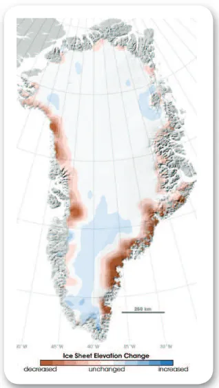
Figure 4. 13 The change of the ice-covering layer on Greenland based on analysis using satellite IceSAT (source: Earthobservatory, NASA, 2007)
Figure 4. 14 The sea level rise until year 2100, relative to sea level in 2000
Figure 5. 1 An illustration of the scheme and causes of marine transportation accidents in the last few decades. SSH and SST indicates the sea surface height and sea surface temperature respectively.
Figure 5. 2 Sea level climatology based on tide gauge, altimeter, and IPCC model data. Model data were only displayed by sea level at the southern coast of Lombok Island.
Figure 5. 3 Result of wavelet analysis for historic data from 1871 to 1998. The dC indicates the degree Celsius
Figure 5. 4 Wavelet analysis results for the SRESa1b scenario. The dC indicates the degree Celsius
Figure 5. 5 Wavelet analysis results for the SRESa2 scenario. The dC indicates the degree Celsius
Figure 5. 6 Wavelet analysis results for the SRESb1scenario. The dC indicates the degree Celsius
Figure 5. 7 Time series of altimeter sea level anomaly from 1993 to 2008. Sea level anomaly falls to 20cm during strong El Niño, and rise 20cm during strong La Niña Figure 5. 8 Hovmoller diagram of time-latitude sea level anomaly from 1993 to 2008, with
lowest sea level anomaly in 1997/1998 during strong El Niño and the highest in 2008 during La Niña
Figure 5. 9 Average of signiicant wave height processed from altimeter from 2006 to
2008
Figure 5. 10 Hovmoller Diagram of daily time-latitude Signiicant Wave Height (SWH)
with the lowest SWH happening in the area at 8°S to 4°N, also SWH height
is inversely proportional between SWH in the South China Sea, Paciic and
Sulawesi Sea (between 4°N to 12°N) with SWH in the Indian Ocean (between 8°S to 12°S)
Figure 5. 11 Maximum signiicant wave height during extreme wave, processed from the altimeter data of signiicant wave height from 2006 to 2008
Figure 5. 12 Time-series of wave height from January 1st 2006 to March 1st 2009 in Java
Figure 5. 14 Wind speed and direction on December 29th 2009
Figure 5. 15 SST anomaly from 90°E to 150°E and from 15°S to 15°N on August and September year 1980 to 2008. The increase of SST of more than 0.35°C shows strong La Niña period, and decrease of 0.35°C shows strong El Niño
Figure 5. 16 Chlorophyll-a distribution on September during normal condition, El Niño and La Niña
Figure 5. 17 Estimated locations where massive coral bleaching happens based on the difference of the highest sea level temperature to mean sea level temperature Figure 5. 18 Coral bleaching sites as a result from SST increase in 1998 until 2006 (Marshall
and Schuttenberg, 2006)
Figure 5. 19 Map of coral reef damage and coral bleaching based on data from Basereef. org
Figure 6. 1 Flow chart of process and general method for estimating sea-water-inundated area in year 2100
Figure 6. 2 Estimation of sea-water-inundated area due to inluence of sea level rise which
reach 1m, subsidence level of 3m per century, and 80cm of tide.
Figure 6. 3 Estimation of sea water-inundated area due to inluence of sea level rise that
reaches 1m, subsidence level of 2m per century, and 50cm of tide.
Figure 6. 4 Estimation of sea water-inundated area due to the inluence of sea level rise that
reaches 1m, subsidence level of 2.5 m per century, with highest tide as high as 1.5 m from MSL.
Figure 6. 5 Inundated area in Jakarta in year 2100 during extreme weather Figure 6. 6 Inundated area in Semarang in year 2100 during extreme weather Figure 6. 7 Inundated area in Surabaya in year 2100 during extreme weather
LIST OF ABBREVIATIONS
CGCM Coupled General Circulation Model
ENSO El Niño Southern Oscillation
GCM General Circulation Model
GISS Goddard Institute for Space Studies
GHG Green House Gases
HYCOM HYbrid Coordinate Ocean Model
IOSEC Indian Ocean South Equatorial Current
IPCC Intergovernmental Panel on Climate Change
ITF Indonesian Through Flow
MODIS Moderate Resolution Imaging Spectroradiometer
MRI Meteorological Research Institute
NASA National Aeronautics and Space Administration
NOAA National Oceanic and Atmospheric Agency
1.1 Background
It has been estimated that 23% of the world’s population lives within both 100 km distance from the coast and less than 100 m elevation above sea level, and population densities in coastal regions are about three times higher than the global average (Small and Nicholls, 2003). This causes a serious vulnerability to the sea level rise caused by global warming. Meanwhile, human activities, in general, are believed to be the biggest contributors to the atmospheric built of greenhouse gases (GHGs), including water vapor (H2O), carbon dioxide (CO2), methane (CH4), and chloroluorocarbons (CFCs).
As the global warming process intensiies, the frequency of occurrence and intensity of El Niño and La
Niña also increases (Timmerman et al, 1999). In general, El Niño occurs once in 2-7 years, but since 1970, the El Niño and La Niña frequency changes to once in 2-4 years (Torrence and Compo, 1999). Moreover, during El Niño in 1997/1998, Indonesia as a whole experienced a long dry season and during La Niña in 1999, Indonesia experienced a high increase of rainfall, with sea level rise ranging from 20 cm up to 30
cm. This combination of events led to loods in large areas of Indonesia, especially in the coastal region. Using sea level data on Java Sea from IPCC models, Soian (2007) Predicted that the frequency of El
Niño and La Niña events will become biennial during the period from year 2000 to 2100.
Aside from extreme climate events (e.g., El Niño and La Niña), global warming also causes sea level rise, both from the expansion of seawater volume as the result of temperature rise in the ocean and from the melting of glaciers and polar ice caps in the North and South Pole. Although the impact of sea level rise is only a subject of discussion among scientists, various climate change studies show that the sea level rise potential could range from 60 cm up to 100 cm, in year 2100. Regardless as the debate people living in the coastal area of Indonesia must have a broad awareness of the decrease of life quality in coastal regions due to sea level rise.
Globally, sea level rise (SLR) is about 3.1mm/year today, while the average sea level rise in the 20th century is only 1.7 mm/year. More than a third of sea level rise is caused by the melting of icecaps in the Greenland and the Antarctica, and by the retreat of glacial ice. Some recent research shows that the
melting of glacial and polar ice will increase as global warming intensiies. If the warming and the melting
of ice continue at a rate similar to that of the past 5 years, then the predicted sea level rise in 2100 could be as much as 80 cm to 180 cm.
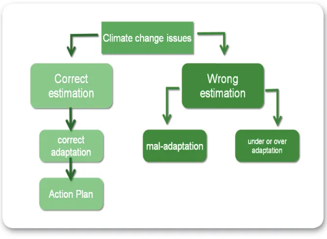
The impacts and the consequences of SLR in various coastal regions will be inluenced by numerous
coastal environments. One approach to understanding the correlations among climate change, adaptation study, and the planning of prudent response strategies are illustrated in Figure 1.1.
Figure 1. 1 Flow chart of climate change study to support for climate change adaptation action plan
1.2 Aims and Objectives
The aims of this study are as follows:
1. To investigate the SLR rate caused by the global warming.
2. To investigate the impacts of global warming on the sea surface temperature (SST), the intensity of
extreme events and their impacts on the signii cant wave height characteristics.
Meanwhile, the purposes of this study are:
1. To provide a base reference and information for resilient coastal area development, in order to adapt to the risks of future climate change, particularly sea level rise (SLR).
analysis for extreme events was conducted using wavelet analysis to i nd the moment and frequency of
occurrences of El Niño and La Niña.
This study is structured as follows: the i rst chapter contains an introduction that includes the background
and objectives of the study; the second chapter outlines the climate and oceanographic condition of Indonesian Seas. It covers sea level and surface temperature climatology, chlorophyll-a spatial distribution, and wave height. The third chapter explains the methodology and the data used for our analysis, while the fourth chapter presents the projection of sea surface temperature (SST) and sea level. It is followed
by the i fth chapter on ENSO projection, based on sea surface temperature in the Nino3 area (dei ned
CLIMATE AND
OCEANOGRAPHIC
CONDITION IN
INDONESIAN SEAS
Indonesia is a maritime country located between two oceans, the Indonesian Ocean and the Paciic
Ocean. This unique geophysical position affects the monsoon pattern, rainfall, and other characteristics of regional climate.
2.1 Wind and Rain Patterns
In the northwesterly wind season from October to March (i.e., when wind blows from the west), the weather in Indonesia is affected by the northwest monsoon. During this period, the wind blows from the northeast and turns to the southeast after passing through the equator. By contrast, in the season of the southeasterly wind from May to September, the wind blows from southeast and turns to northeast after
passing through the equator. The inluence of the Paciic Ocean is dominant in the period of westerly
wind (except in most part of Sumatera, which is affected by the western Indian Ocean). Meanwhile
during the season of the easterly wind, the inluence of the Indian Ocean is dominant, and is marked
by reduced rainfall on Java Island and in Nusa Tenggara. However, during this period, most parts of Sumatera and Kalimantan still have high probability of experiencing medium intensity of rainfall.
The propagation of northerly wind from October to March pushes down the warm seawater from the
Paciic Ocean to the Indian Ocean. This causes high rainfall in almost every area of Indonesia. While in
the season of easterly wind from May to September, eastern wind pressure pushes the low temperature
seawater back from the Indian Ocean to the Paciic Ocean through the Java Sea, the Karimata Strait
and the South China Sea. This period is marked by decreasing rainfall in Java, Kalimantan and southern Sumatera. At the same time, in the Riau Islands, western Sumatera may still have rain due to the high SST around those areas.
a. January b. August
Figure 2. 1 The pattern of wind and sea level temperature (SLT) in January and August
a. January b. August
Figure 2. 2 Annual cycle of mean rainfall in Indonesia in January and August
2.2 Sea Level Variations
2.2.1 Ocean Currents and Sea Level
Generally, the pattern of Indonesian Through Flow (ITF) affects the climate characteristics of the region
through the heat-transfer mechanism between Pacii c Ocean and Indonesian Seas. Figure 2.3 shows surface l ow and spatial distribution of sea level on January and August. Flow pattern and sea level
estimation have been calculated using HYbrid Coordinate Ocean Model (HYCOM, Bleck 2002). The
a. January b. August
Figure 2. 3 Spatial distribution of SLH and surface current in January and August. SLH is based on altimeter data, while the direction and the speed of current is an estimation result using HYCOM
(HYbrid Coordinate Ocean Model) (Soi an, 2007)
In general, sea level in Indonesian waters is high in January (northwest monsoon) and low in August
(southeast monsoon). Meanwhile the yellow lines and arrows in Figure 2.3 illustrate the surface l ows
of the Indian Ocean South Equatorial Current (IOSEC). Each of the white and solid red line and
arrow illustrate the Indonesian Through Flow (ITF) from the South Pacii c to Indian Ocean, through
the Makassar and Lombok straits, and also the South China Sea, Karimata Strait, and Java Sea. The red
dotted line and arrow indicate the surface l ows of the Pacii c South Equatorial Current (PSEC), with
SEC and ITF sketches based on Vranes et al. (2003). In the period of west monsoon, i.e., January, Figure 2.3 (a.) illustrates that the IOSEC move westward in the region of 10°S to 20°S, while mesoscale eddies are not clearly seen in the South China Sea. The strong surface current in the South China Sea causes the increasing sea level from western and northern Kalimantan to eastern Vietnam. Then the PSEC located
between latitude 5°N to 15°S until 20°S l ows westward due to the blowing of the Pacii c Trade Wind (PTW) from the aquatic zone around Peru to longitude 180°E. Meanwhile, the Pacii c North Equatorial
Current (PNEC), which is normally located between latitude 10° to 25° N, is heading westward by the southeasterly trade wind. When PNEC reaches the Philippines, this surface current is broken, with the
smaller part moving to the south to form the Pacii c Equatorial Counter Current (PECC), while the
biggest part moves to the north to form the Kuroshiyo current. In addition, the current in Makassar Strait weakens due to the strength of the surface current of the Java Sea.
Ocean through the Lombok Strait.
Figure 2.4 shows the pattern of monthly average surface current and sea level over a period of 7 years from 1993 to 1999, measured in January and August. Current pattern and sea level height estimation
based on the HYbrid Coordinate Ocean Model (HYCOM, Bleck 2002). Model coni guration for the Java Sea, Makassar Strait and most parts of the South China Sea is outlined in Soi an et al, (2008).
a. January b. August
Figure 2. 4 Distribution of sea level and surface current pattern in January and August. The sea level and the current pattern are the monthly average in 7 years, from 1993 to 1999
Figure 2.4 (a) shows the current patterns in January during the southwest monsoon. The propagation
of southwesterly wind causes the current in the Java Sea to l ow eastward and the water from the Indian
Ocean enters into the Java Sea via the Sunda Strait. The topographic effect of the shrinking and shallowing of the southern Karimata Strait’s depth, causes a 40 cm of sea level difference between the Java Sea and the Karimata Strait. Moreover, the current pressure to the east causes the gradient of sea level height difference, with a decreasing of sea level height in the Java Sea and an increase of the sea level in Banda Sea, as well as along the northern coast of Lombok Island (as can be seen for January in Figure 2.4). These wind patterns change as the seasons change. The wind that blows from southeast in the dry season (i.e., during the southeast monsoon) pushes the current in the Java sea to the west, while the current in
Karimata strait moves to the north (Figure 2.4). The Java Sea surface water then l ows out through Sunda
Strait as seen in Figure 2.4.
surface current in the Makassar Strait strengthens in the dry season (with the southeasterly wind), and pushes the low salinity and temperature surface water back to the Java Sea. The strong Makassar Strait
surface l ow also causes the decreasing of sea level along the northern coasts of Lombok Island, Flores
Sea, eastern and middle Java Sea on August, as seen in Figure 2.4 b).
2.2.2 Tidal Forcing
The OTIS model is calculated based on assimilation between the tide gauge and altimeter data from October 1992 to December 2008. Moreover, the average of the highest tidal range is depicted in Figure 2.5.
Based on OTIS model for Indonesia, it is known that the highest tidal range occurs in the southern coast of Papua Island that reaches 5 m, with each highest and lowest tide is about 2.6 m to -2.6m. The Southern Karimata Strait has the tidal range between 2.2m and 2.4m, with highest tide reaches 1.2m, and lowest tide between -1.1 m and 1.1 m. The tidal range height in Java Sea is about between 1.2 m and 2m, with the highest tidal range in the eastern Java Sea around Surabaya, Madura, and Bali. It is also seen that there is a time difference of the highest tide occurring in the Java Sea, with the highest tide is in around Jakarta, occurring in 00.00 WIT until 01.00 WIT, and then shifted to the east, with the highest tide is around Bali
in 12.00 WIT (i gure not shown).
Figure 2. 5 Spatial distribution of the monthly mean highest tidal range in the Indonesian Seas
2.2.3 Signifi cant Wave Height
Figure 2.6 illustrates a 3-year average of wave height data for January and August that was obtained from
altimeter data of Signii cant Wave Height (SWH). The average wave height in January ranges from about 60cm to 240cm, with the highest waves reaching 3m and occurring in the West Pacii c, in north of Papua.
The wave height characteristic over the north of equator has the highest annual wave during January, except along the west coast of Sumatera where it is bordered by the Indian Ocean.
a. January
In contrast, the area that is located south of the Equator has the highest annual waves in July and August. In addition, the highest waves in August occur in the Indian Ocean, with the height exceeding 3m, whereas the wave height in the Makassar Strait, the Karimata Strait, and the aquatic around Ambon island, have the lowest wave height, with a range of about 60 cm to 1 m. In addition, the wave height in Java Sea reaches its highest point in July to August, with a range of about 1.2 m to 1.4 m.
2.3 The Distribution of Chlorophyll-a and Sea Surface Temperature
Along with the seasonal wind pattern, the spatial distribution of chlorophyll-a in January and August is shown in Figure 2.7, based on the Seawifs data. Generally, the chlorophyll-a concentration is low in January in northwest monsoon, although medium and high concentration of chlorophyll-a is still seen in West Kalimantan, Riau Islands and Java Sea. However, it shows high turbidity level due to the wind propagation that causes the perfect mixing layer formation to the bottom. This is because of the Java Sea, Riau Island and South Karimata Strait have average depth less than 50m.
b. August
Figure 2. 7 The spreading pattern of chlorophyll-a in January and August
The chlorophyll-a concentration in the deep ocean such as the Indian Ocean of south Java Island is decreasing because of the down-welling due to the propagation of westerly wind. SST increases due
to the warm water of sea level from the Pacii c Ocean (Figure 2.1). This causes a decrease in i shing
potential. Meanwhile, in August it increases especially in Indian Ocean, because the upwelling process is getting intensive due to the strong easterly wind. The concentration of chlorophyll-a is concentrated in the Indian Ocean south of Java Island with a concentration of more than 3mg/m3. Moreover, the
i shing potentials in the Java Sea and the Riau Islands water are also increasing, due to the transfer of
3.1 Data
Sea level data used in this study includes:
1. Historical data consisting of:
• Tidal data which was compiled from the following stations: Surabaya, Benoa, Darwin, Broome, Ambon, Singapore, Jakarta, Bitung, Sibolga, Manila and Sandakan. Monthly sea level average is
deined as sea level during that month minus average sea level for the period of observation. All
tidal data is obtained from the UHSLC (University of Hawaii Sea Level Center). Figure 3.1 shows time-series data for monthly sea level from several tide gauge stations.
• Altimeter data from several satellites have been merged for this study. Altimeter satellites used for this study include TOPEX/Poseidon (T/P), GFO, Envisat, ERS-1 and 2, also Jason-1, that is provided since October 1992 to October 2008. The altimeter data for this study was obtained from AVISO (AVISO, 2004).
2. Model output data for the period of 2000 - 2100 was obtained from the IPCC Special Report on Emission Scenario (SRES), focusing on scenarios b1, a1b and b2. These scenarios project CO2 concentration in 2100 of up to 750 ppm (part per million by volume) and 540 ppm. For this study, the primary emphasis has been placed on the analysis results using the Scenario a1b SRES. The IPCC data used for this analysis include the data for sea surface temperature and sea level, along with the output data from MRI_CGCM2.3 (Japan), CCCMA_CGCM3.2 (Canada), Miroc3.2 (Japan), and NASA GISS ER (USA) model.
3. Supporting data used in this study include:
• Data on sea surface temperature derived from NOAA (National Oceanic and Atmospheric Agency) OI (Optimal Interpolation) (Reynolds, 1994) for the period of 1981 until 2008.
Figure 3. 1 Example of time-series of Sea Level Data from several stations in Indonesia and surrounding area.
3.2 Method
For this study, the method used to estimate sea level rise and the occurrence of extreme events (e.g., El Niño and La Niña), involve:
1. Trend analysis to expose the tendency and rate of sea level rise based on the historical data, including altimeter satellite data and tide data, along with the IPCC modeling output data. In this case, the trend analysis was developed as a linear regression of sea level by month, with the following mathematic equation of y = a + bt,
Where y is sea level, t is time stated in months,
a is offset, and b is the rise rate (slope, trend).
Figure 3. 2 Flowchart of sea level rise estimation using historical data and IPCC model, which consists of 4 models, which are MRI, CCCMA CGCM 3.2, Miroc 3.2 and NASA GISS ER
2. Composing climate data to i gure out the effect of monsoon to the characteristic of
Figure 3. 3 Climatology of sea level based on tide data, altimeter and model
non-stationary phenomena (signal with changing frequency). The wavelet transformation approach has several advantages compared to the alternative Fourier transformation that is frequently used. By comparison, Fourier transformation can only be used to detect stationary phenomena (signal with constant frequency).
The time and frequency of ENSO occurrence can be determined by using wavelet analysis of SST
in East Pacii c. The SST is dei ned between 150°WL (west longitude) to 90°WL and from 5°NL
(North Latitude) to 5°S (South Latitude), which is sometimes referred to as the Nino3 area. The application of this process to Nino3 area in order to create the ENSO index is shown in Figure 3.5. An example of applying the detection process to an extreme climate event is illustrated in Figure 3.6. Details of the explanation concerning extreme climate events are described in Chapter V.
2 The calculation of tidal forcing is done by using an OTIS (Ocean Tidal Inverse Solutions) that we acquired from the Oregon State University. The OTIS is based on the altimeter data for the year 1992 to 2008, primarily with emphasis to the TOPEX/Poseidon data. The OTIS calculation is built using a method of assimilation for both altimeter and tidal gauge data. The numerical algorithm and mathematical equation used in the OTIS model is shown in Egbert, et al. (1994). OTIS has several advantages compared to pure tidal gauge data. Most importantly, it can predict the current and height of tides in the open sea with high accuracy. An example of sea level calculations based on an OTIS model is shown in Figure 3.7. Meanwhile, the tidal data for the same period is illustrated in Figure 3.8. In addition, a validation test between the OTIS model run and tidal station data for Jakarta is shown in Figure 3.9. This analysis applies tidal prediction process using 8 main harmonic constants, namely O1, K1, M2, S2, N2, Q1, P1, and K2. Validation test result shows that the OTIS output has a correlation up to 0.7 with Root Mean Square Error (RMSE) up to 10 cm.
]
Figure 3. 6 Wavelet analysis result using Nino3 SST data and results from the MRI model for SRESa1b scenario
Figure 3. 8 Speed and direction of tidal current at07.00 WIT when is heading to the lowesttide
PROJECTION OF SEA
LEVEL RISE AND
SEA SURFACE
TEMPERATURE
Global warming resulted from the atmospheric buildup of greenhouse gases has an important effect on sea level. In general, the gradual increase of sea level caused by global warming is one of the most
complicated aspects of the global warming effect, as its acceleration rate is a function of the intensii cation
of global warming. Sea level rise is affected by the addition of water mass, which results from the melting of glaciers and ice sheet in the Greenland and the Antarctica, as well as from the increase in water volume
due to thermal expansion of the upper mixed layer (with i xed water mass), which is caused by the rising
water temperature. This chapter explains the projection of SST and sea level rise based on the NOAA OI SST, tidal and altimeter data, and model results from the IPCC portal.
Figure 4. 1 Time-series of SST data based on paleoclimate data from 150 thousand years ago to 2005,
with the highest SST occurring 125 thousand years ago, 30ºC in the West Pacii c and the Indian Ocean, and 28 ºC in the East Pacii c (Hansen, 2006)
4.1 Sea Surface Temperature Rise Projection
Based on the paleoclimate data of the Pacii c and Indian Ocean (Figure 4.1, Hansen, 2006), it can be
deduced that the highest sea surface temperature occurred 125 thousand years ago, when the sea reached
30ºC in the West Pacii c and Indian Oceans, and 28 ºC in the East Pacii c Ocean. From Figure 4.1, it can
Figure 4. 2 The trend of SST rise based on the data of NOAA OI, with the highest increase trend
occurring in the Pacii c Ocean in the north of Papua, and the lowest in the south coast of Java.
The modern record of SST is based on the monthly SST data provided by the U.S. National Oceanographic and Atmospheric Agency (NOAA). The primary dataset is the Optimum Interpolation (OI) version 2 (Reynolds, 1994), from year 1983 to 2008, as shown in Figure 4.2. Figure 4.2 illustrates the variation of SST rise rate of -0.01°C/year to 0.04°C/year, where the highest trend occur off the northern coast of Papua Island, and the lowest one occur on the south of Java Island. However, this negative trend does not indicate the long-term SST changing rate within this area for the future. This negative rise rate could have been caused by the increasing frequency of El Nino and the elevated wind speed coming from the southern Indian Ocean, which will be explained in Chapter V.
For comparison, the average trend of the SST rise rate in the Indonesian waters ranges from 0.020°C/ year to 0.023°C/year. Based on this, it can be concluded that the SST in year 2030 will reach 0.6°C to 0.7°C, and will reach 1°C to 1.2°C in year 2050, relative to the average SST in 2000. In addition to that, SST is expected to rise by 1.6°C to 1.8°C in year 2080, and could reach 2°C to 2.3°C in year 2100. This would indicate that the projected SST in 2050 is the highest temperature during the last 150 thousand
years, when compared to SST detected in paleoclimatic data for the western Pacii c Ocean.
Figure 4. 3 The global trend of SST based upon observation data from 1870 to 2000, with the rate of SST rise reaching 0.4°C/century±0.17°C/century (Rayner, et al., 2003)
Figure 4. 4 The rate of SST rise based on IPCC SRESa1b, using the MRI_CGCM 3.2 model
Table 4. 1 Projection of the SST increase of Indonesian waters
Item 2030 2050 2080 2100 SRESa1b 0.65°C 0.65°C 1.10°C 1.10°C 1.70°C 1.75°C 2.15°C 2.20°C
Level of
Coni dence High High High High
Finally, high SST rise will affect the potential i shing ground and the damage of coral reefs. The i shing
ground probably will move from the tropical area of Indian Ocean, Banda Sea, and Flores Sea, to the sub-tropical areas that remain at lower temperature. On the other hand, if the SST rise rate stays within the adaptive capacity of the reefs and other coastal life forms, then the damaging effects on coastal ecosystems caused by SST rise may be avoided. In addition, as the sea-surface temperature increases, sea level will also rise due to the process of thermal expansion and the adding of water mass from the melting of glacial ice and icecaps in the Greenland, and the Antarctica. The potential sources for sea level rise are depicted in Table 4-2.
Table 4. 2 Potential sources of the sea level rise
Potential source of the sea level rise
4.2 Sea Level Rise Projection
4.2.1 Sea Level Rise Projection based on the IPCC AR4
The average sea level in the Indonesian Seas is shown in Figure 4.5. Generally, the sea level in the Pacii c
Ocean is 30cm to 50cm higher than that of the Indian Ocean. Sea level in the Java Sea ranges from 20cm to 30cm and 30cm lower than the one over the Karimata Strait. The pattern of Indonesia Through Flow (ITF) can clearly be observed from the characteristics of sea level, forming a lower sea level than that around it, especially the central ITF pathway through the Makassar Strait and point towards the Indian Ocean through the Lombok Strait, the Timor Strait, and the Savu Sea. Even so, the eastern ITF pathway is also visible across the Maluku Archipelago, pointing towards the Indian Ocean through the Timor Strait and the Savu Sea. On the other hand, the western ITF pathway across the Karimata Strait, the Java Sea, and the Lombok Sea cannot be clearly seen. This may be caused by the current of both straits which
is mainly inl uenced by wind, with the depth of 40m to 50m, even though the usual annual current tends to l ow towards the Indian Ocean across the Lombok Strait (Soi an, 2008). Details about the seasonal
current pattern are discussed in Chapter II.
Figure 4. 5 Average sea level rise for 15 years from January 1993 to December 2008, using 0 cm as the lowest regional sea level
Sea level rise due to global warming will bring inevitable consequences. Seasonal current patterns and
ITF might be inl uenced by the changeable rise of sea level, particularly in areas where the rise of Pacii c
alteration, and the reduction of wetland area in coastal zones. Wetland ecosystems in coastal zones might be damaged if the rise of sea level and SST exceeds the maximum limit of adaptive capacity of coastal life forms. Moreover, the rise of SST also increases the rate of intrusion by seawater into the coastal environment.
To investigate the impacts of global warming on sea level rise rate and its characteristics, the comparative analysis is used to compare the average sea level from 1993 to 2000 with the one from 2001 to 2008. These results can be combined with the use of spatial trend analysis using the data from 1993 to 2008. Figure 4.6 shows the change of sea level based on altimeter data by using the comparative analysis for
7 years. The highest sea level rise rate occurred in the western part of Pacii c Ocean with 8 cm rise; the
smallest increase occurred in the area off the south coast of Java Island, South China Sea, and the west coast of Philippines near the site of the Mindanao Eddy. Meanwhile, the low sea level rise near the south coast of Java Island is strongly correlated with the thermal expansion caused by temperature in these
regions. In general, the differences in sea level rise between the Pacii c and Indian Ocean may change the
ITF characteristics. These changes will possibly alter the regional climate of Indonesia. The rise of sea
level in the Pacii c Ocean, which is higher than that of the Indian Ocean, enhances the water transport intensity of warm water from the Pacii c to Indian Ocean. Eventually, the increasing intensity of ITF
could cause a change in the local rain patterns all over Indonesia.
Figure 4. 6 The average magnitude of sea level from 2001 to 2008 subtracted from the average magnitude of sea level rise from 1993 to 2000, with the varying increase of sea level between 2 cm and
2030, with the average SLR for all of Indonesia ranging from approximately 15 cm to 18 cm. By 2050, SLR could reach 10 cm to 50 cm, with an average of 25 cm to 30 cm. SLR in 2080 could reach 16 cm to 80 cm with an average ranging from 40 cm to 48 cm. By the end of the century, sea level rise could range from 20 cm to 100 cm, with an average of 50 cm to 60 cm.
Figure 4. 7 The trend of sea level increase based on altimeter data from January 1993 to December 2008 using spatial trend analysis
Figure 4. 8 Approximation of sea level rise using a number of tidal data acquired from the University of Hawai’i Sea Level Center (UHSLC)
Figure 4. 9 Approximation of global sea level change based on the IPCC SRESa1b assuming CO2 concentration of 750ppm
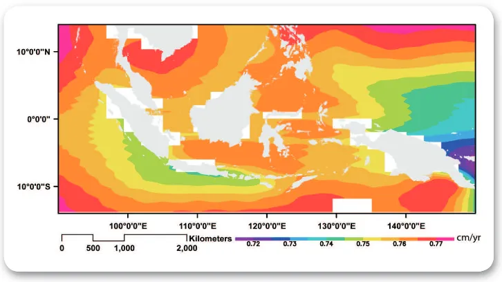
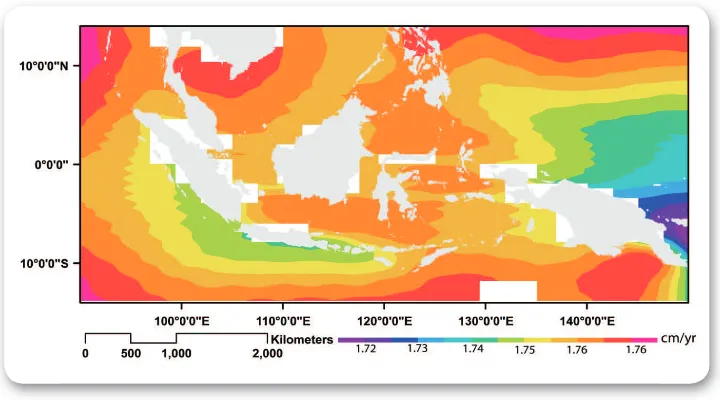
Figure 4.10 shows the spatial distribution of the sea level rise based on the MRI 3.2 model applied to the global climate described in the SRES A1b scenario. Sea level rise based on the model has smaller projected range than the altimeter-based projection does, although it possesses a relatively similar spatial
distribution signii cant differences occurring only in the northern Indian Ocean. The narrow range of
the model-based projections of sea level rise rate might be caused by the low spatial resolution of the global model. The rate of sea level rise is projected to range from 0.7 cm/year to 0.8 cm/year. Overall, average sea level is projected to rise by 22.5 cm ±1.5 cm in 2030 relative to the sea level in 2000. By 2050, the cumulative rise is expected to range from 35 cm to 40 cm. Sea level is projected to continue rising, reaching 60 cm ±4 cm in 2080, and 75 cm ±5 cm in 2100.
Figure 4. 10 Approximation of the amount of sea level rise in the Indonesian waters based on the scenario of IPCC SRESa1b, assuming CO2 concentration of 750ppm
The estimation of sea level rise using altimeter, tidal, and model data shows the same trend, with the average rise rates ranging from 0.6 cm/year to 0.8 cm/year. The summary of sea level rise from 2030 to 2100 relative to sea level in 2000 is illustrated in Table 4-3.
Table 4. 3 Projection of the average increase of sea level in the Indonesian waters
Period Sea Level Rise Projection since 2000 Level of
coni dent greenhouse gases (GHGs) during the last 50 years has been caused by human activity. These increases of GHG concentration are likely to lead not only to an increase of air and SSTs, but also to an increase of sea level through thermosteric process. Moreover, this increase in concentration caused the increase of global temperature, especially in the Greenland and the Antarctica, and in the central Siberia. In addition, the increase of sea level will range from 20 cm to 80 cm, according to the analysis contained in the IPCC AR4. However, the NASA GISS E_R model projects a 90 cm increase of sea level by year 2100. The IPCC AR4 analysis allocates 70% of this sea level rise to thermosteric processes and 30% to the melting of glacial ice. Meanwhile, the research completed in 2005 has showed an increasing intensity of ice melting, in both the Antarctica and the Greenland.
.
Figure 4. 11 Positive feedback of ice melting and the rising of surface temperature (UNEP/GRID-ARENDAL, 2007)
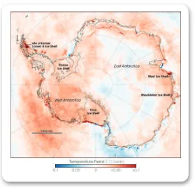
Figure 4.12 depicts the surface temperature change in the Antarctica for the last 30 years, with the average rise rate ranging from 0.05°C/year to 0.1°C/year. The highest rise rate of surface temperature occurred in the western Antarctica, contributing the potential addition of 6 m to 7 m of sea level, if all surface ice melts. Global sea level rose 1.7± 0.5mm/year until the end of the last century. This is different compared to the global SLR between 1993 and 2003, when the average rate reached 3.1±0.7 mm/year. The change of rise rate indicates the increasing of long-term rise rate variability. This fact indicates that both temperature and ice-lost are contributing to the SLR. However, the model and IPCC AR4 approximation shows no indication of dynamic alteration of ice melting.
Figure 4. 12 The change in Antarctica’s temperature in the last 30 years (Source: Earthobservatory, NASA, 2007)
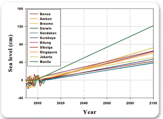
Rahmstorf (2007) use the relationship between the rise of the sea level and surface temperature to predict the sea level rise in the end of the 21st century. His estimate ranges from 50 cm to 140 cm, relative to the sea level in 1990. This prediction is higher than the projection of IPCC AR4. Moreover, the sea level rise before 1990, due to mass changing, is purely dominated by the glacial melting (Bindoff, et al., 2007), thus Rahmstorf ’s prediction (2007) excludes the changing of sea level due to the ice melting in the Antarctica and the Greenland.
Figure 4. 13 The change of the ice-covering layer of Greenland based on analysis using IceSAT satellite (source: Earthobservatory, NASA, 2007)
Figure 4. 14 The sea level rise until year 2100, relative to sea level in 2000
EL NIÑO AND LA NIÑA
PROJECTIONS
It cannot be denied that in the last few decades, many natural disasters have occurred, including coastal
l oods, ship accidents and tidal waves caused by extreme weather events. The extreme weather conditions, possibly associated with El Niño and La Niña in the Pacii c Ocean along with the Indian Ocean Dipole
Mode (IOD) in the Indian Ocean, have direct effects on coastal zones and marine transportation, as well as indirect effects on the forestry, agriculture, health, and land transportation sectors, through changes in rainfall caused by extreme weather.
Many oceanographers believe that with the increasing intensity of global warming, the intensity of extreme events such as El Niño and La Niña (usually known as ENSO, or the El Niño-Southern Oscillation, comprising both El Niño and La Niña) will increase as well. ENSO is a natural phenomenon occurring
every few years, because of the evolution of SST in the tropical Pacii c Ocean. El Niño is marked by the
decrease of SST in the Indonesian waters, and an increase of more than 0.5°C in the eastern tropical
Pacii c Ocean. As a consequence, the air pressure in Indonesia rises, causing the Pacii c trade wind to
weaken and easterly local winds to strengthen, although, in the early phases of El Niño, westerly local wind bursts are also known to happen. The decreasing of SST and the shifting of the warm-pool from the
Indonesian waters to the central tropical Pacii c Ocean, cause a decrease in rainfall in most of Indonesia. This, in turn, increases the risks of forest i res and drought, especially in the eastern Indonesia. On the
other hand, La Niña is a natural phenomenon with dynamics and impacts that are opposite to El Niño.
La Niña is marked by the rise of SST in the Indonesian waters, and the fall of SST in the eastern
tropical Pacii c Ocean by more than 0.5°C. In the La Niña period, the Pacii c trade wind becomes more
intense, which causes the pool to shift to the west compared to normal conditions. This warm-pool westward shifting causes more intense rainfall in Indonesia, and therefore increases the dangers of
l ooding.
Aside from forest i re and l ood risks, ENSO can also assist in causing tidal waves and tropical storms, which may cause coastal l ooding and marine transportation accidents. An illustration and the mechanism
Many of the sea transportation accidents that have occurred recently were caused by high waves and ocean winds resulting from extreme weather (e.g., the KM Senopati disaster on December 29, 2006, and the KM Teratai Prima on January 11, 2008). However, other factors such as tidal and wind-induced surface currents were also involved in these accidents.
5.1 Global Warming and ENSO
The ENSO phenomenon is based on the changing patterns of ocean surface temperatures in the Pacii c
Ocean. Therefore, the frequency of El Nino and La Nina can be estimated using the data of Nino3 (the
region of the eastern Pacii c Ocean spanning from longitude 210°E to 270°E and from latitude 5°S to
5°N) SST, by using wavelet analysis. The SST data of Nino3 is in turn obtained from MRI models. (The choosing of model is based on climatologic comparisons of the most realistic sea levels in the case study in the Lombok Island, Figure 5.2). The SST data of Nino3 used are monthly anomaly data.
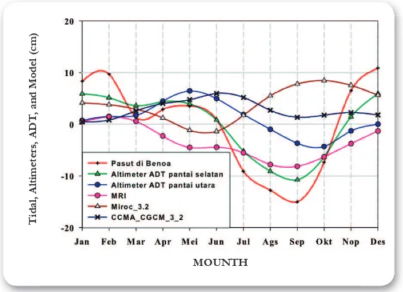
Figure 5. 2 Sea level climatology based on tidal gauge, altimeter, and IPCC model data. Model data were only displayed by sea level at the southern coast of Lombok Island.
Figure 5.2 shows the sea level climatology with tidal gauge, altimeter, and IPCC model data. The MRI 3.2 model shows a sea level estimation, which is more realistic compared to the highest yearly sea level occurring in January to February, and the lowest occurring in August to September. The Absolute Dynamic Topography (ADT) altimeters on the southern coast of Lombok showed the same pattern as the estimation of MRI 3.2 with the highest sea level occurring in January to February and the lowest
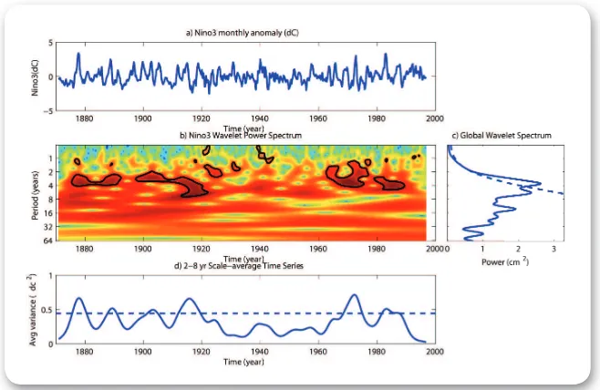
Figure 5.3 shows the results of the wavelet analysis using historic data from 1871 to 1998. Based on the historical data of Nino3 SST from 1870 to 1998, it has been shown that ENSO occurs every two to seven years, with an intensive ENSO period occurring from 1875 to 1885 at the beginning of the industrial revolution in Europe. The second ENSO period occurred in 1900 to 1920, during the First World War. The third period occurred from 1920 to 1939, with a frequency of one to two years. This is correlated with the mass industrialization put in action, especially by the defeated nations in the First World War,
followed by the ENSO period from 1939 to 1945 with a one-year frequency for i ve years. The ENSO
phenomenon entered a relaxing period from 1945 to 1965, which was followed by the fourth period from 1965 to the present day. The increasing frequency of ENSO since 1965 is caused by the development of Third World countries, changing from agrarian to industrial countries. After 1965, the ENSO period has risen to once every two to six years with a longer length of time. The total power spectrum energy shows that the ENSO with a frequency of four years has the highest energy (see panel c). This shows that from 1870 to 1999, the average frequency of the occurrence of ENSO is around four years.
Figure 5. 3 Result of wavelet analysis for historic data from 1871 to 1998. The dC indicates the degree Celsius
20 cm. Aside from the rising sea levels; extreme climate conditions will cause extreme weather that may lead to additional high waves.
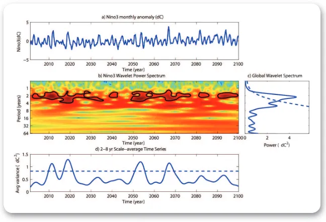
Figure 5. 4 Wavelet analysis results for the SRESa1b scenario. The dC indicates the degree Celsius
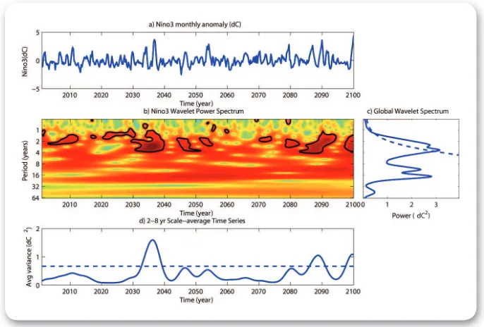
Figure 5.5 shows the result of wavelet analysis applied to the SRES A2 scenario. This analysis indicates the largest El Nino and La Nina events are projected to occur from 2045 to 2050, 2060 to 2065, and 2075 to 2085. The energy spectrum of SRES A2 is lower than the SRES A1b scenario in the period prior to the year 2050, although ENSO still occurs every three years. (See Figure 5.4 panel c.) But the strength of the ENSO dynamic is lower than that in the SRES A1b scenario. The average frequency of ENSO in this scenario is once every four years, based on global spectrum data (panel c). However, the frequency of ENSO increases drastically after 2060. (See Figure 5.4, panel d).
Figure 5. 5 Wavelet analysis results for the SRESa2 scenario. The dC indicates the degree Celsius
Figure 5. 6 Wavelet analysis results for the SRESb1scenario. The dC indicates the degree Celsius
Table 5. 1 ENSO timetable based on the MRI model output
5.2 ENSO and Sea Level Variations 5.2.1 ENSO and Mean Sea level
Using HYbrid Coordinate Ocean Model and tidal gauge data from Jepara, Jakarta, and Surabaya, Soi an (2008) discovered that ENSO inl uence is still clearly seen using the model and tidal data. Both model
and tidal data show a drastic and rapid increase during the transitional period between strong El Niño (1997/1998) and strong La Niña (1998/1999). However the model estimates tends to be lower than the observed tide in Jepara and Surabaya.
Figure 5.7 shows the time-series of altimeter sea level anomaly from year 1993-2008. Monthly sea level anomaly is calculated based on the weekly mean sea level at longitude 90°E to 150°E and from latitude 5°N to 5°S, relative to sea level climatology. During El Niño, sea level will be depressed up to 20 cm below normal, and during La Niña it will be elevated by 10 cm to 20 cm. This affects the risk of erosion,
abrasion, and seawater inundation, particularly during La Niña, which brings higher rain intensity. Soi an
et al. (2007) posted that sea level rise during the transitional period of El Niño and La Niña, and during
Figure 5. 7 Time series of altimeter sea level anomaly from 1993 to 2008. Sea level anomaly falls to 20 cm during strong El Niño, and rise 20 cm during strong La Niña
In addition, it is also clearly seen that sea level is highly rising and reaching up to 20 cm from year 1993 to 2008 (although there is a sea level anomaly drops from 1999 to 2004). Since 2004, the sea level rise has been in rebound with a higher acceleration rate. This is noticed by the rising value of sea level during El
Niño. Moreover, the inl uence of geographical location to sea level rise can be seen in Figure 5.8.
Figure 5.8 shows the Hovmoller diagram of sea level anomaly in the Indonesian Water from 1993 to 2008. This diagram displays average sea level anomaly from longitude 90°E to 150°E against the latitude. Based on the Hovmoller diagram in Figure 5.8, the Indonesian Waters located from latitude 10°S to 15°S have a small sea level oscillation compared to the other regions, with the highest sea level anomaly in 1999 and 2006, and ranging from 10 cm to 15 cm. On the other hand, the lowest sea level anomaly occurred during moderate and strong El Niño between 1993 to early 1998, with a range from -10 cm to -5cm. The Java Sea, Karimata Strait, southern South China Sea, Banda, Flores, and Aru Sea, that are located from latitude 10°S and 8°N, have the lowest sea level anomaly that reached to -20 cm in 1997 to 1998, and the highest, reached 20 cm, during January to April 2008.
The northern part of South China Sea and north of Papua, have the highest sea level anomaly with low oscillation level, ranging only from -5 cm to 20 cm. From the abovementioned conditions, it can be concluded that the areas around the equator from latitude 10°S to 8°N is strongly affected by the ENSO in comparison to other regions.
5.2.2 ENSO and Extreme Waves
Generally, the distribution of yearly average signii cant wave height (SWH) in the Indonesian waters can be seen in Figure 5.9. This i gure shows the highest SWH in the Indian Ocean. The average SWH in Java
Figure 5.10 shows the Hovmoller time-latitude diagram of daily wave height in the Indonesian waters
from October 11, 2005, until March 4, 2009. The i gure illustrates the average wave height on the
longitude 90°E to 150°E against latitude. Figure 5.10 shows that the wave height in the Indian Ocean is inversely proportional with the wave height on the north side of equator line in the Indonesian waters. The wave height in the Indian Ocean increases in April to October and tend to decrease in November to March. The Karimata Strait and Makassar, along with the South China Sea and Sulawesi, have the highest annual wave height during the northwest monsoon from October to March and the lowest annual wave height during the southeast monsoon from May to September.
Figure 5. 10 Hovmoller Diagram of daily time-latitude Signii cant Wave Height (SWH) with the lowest
SWH happening in the area at 8°S to 4°N, also SWH height is inversely proportional between SWH in
the South China Sea, Pacii c and Sulawesi Sea (between latitude 4°N to 12°N) with SWH in the Indian
Ocean (between latitude 8°S to 12°S)
On the other hand, the maximum SWH occurs during extreme waves because of the increase in wind forcing, as seen in Figure 5.11. Besides, the spatial distribution of average wave height in the Indian
Ocean is higher than the average wave height in the Pacii c Ocean north of Papua Island, although the extreme wave in the Pacii c Ocean is 1 m to 2 m higher than the extreme wave in the Indian Ocean.
Figure 5. 11 Maximum signii cant wave height during extreme wave, processed from the altimeter data of signii cant wave height from 2006 to 2008
Figure 5. 13 Time-series of wave height from January 1st 2006 to March 1st 2009 in the southern of Java Island
Extreme waves that occur as a result of extreme events may cause sea transportation disasters. Figure 5.12 and 5.13 shows how extreme events such as La Niña and El Niño can cause a wave with variation between 2.1 m and 2.5 m in the Java Sea, and 3 m to 3.5 m in the southern part of Java Island. This
occurs even though El Niño does not impact signii cantly on the wave height along the southern coast
of Java. During El Niño, the air pressure in Darwin increases and causes a decrease of westerly wind speed, but wind bursts (i.e., the momentary impulse of high velocity westerly wind that occurs due to low and unstable SST in Indonesia) often happens in open seas during this period and rarely happens in semi-enclosed regions like the Java Sea. (See Figure 5.14). Anomalies in the wind pattern with two vortex in the Western Kalimantan and Australia can occur during this period, causing high-velocity pulses of western wind in the Java Sea to reach 20 m/s. Increasing wave height in the Java Sea, on December 29th 2006, such a high-velocity pulse occurred, increasing the wave height in the Java Sea and causing the KM. Senopati to sunk, killing more than 200 passengers on board.
Figure 5. 14 Wind speed and direction on December 29th 2009
5.3 ENSO, Sea Surface Temperature and Chlorophyll-a
The displacement of the warm-pool is a good indicator of the multiyear phenomena, El Niño and La Niña. This displacement brings impacts to sea surface temperature in the Indonesian waters. From climatological data (see chapter III), it is known that in August to October during the southeast monsoon, the concentration of chlorophyll-a off the southern coast of Java Island, Nusa Tenggara, southern Sumatera, Ambon and Sulawesi increases, reaching 0.4 mg/m3 as the result of upwelling caused by easterly wind propagation. On the other hand, the sea level temperature reaches its annual lowest point, between 26°C and 27°C.
In general, the i shing grounds are inl uenced by SST and chlorophyll-a concentration (Hendiarti et al., 2005). The i shing ground potential of the area will increase when the SST is low and the concentration
of chlorophyll-a is high as the result of the upwelling that lifts nutrients from deeper layer (100 m to 200 m). These effects combine with lower temperature resulting from the Ekman Pumping effects that
is caused by coriolis force and easterly wind. The upwelling intensii es during each El Niño. In addition,
there are other areas where upwelling occurs because of local Ekman transport, especially in water bodies surrounding the Banda Sea and Flores Sea. On the other hand, the high concentration of chlorophyll-a off the southern Papua coast may not indicate upwelling, but instead illustrate the intensity of abrasion and the turbidity of the sea, as it depth does not exceed 50m.
Figure 5. 15 SST anomaly from 90°E to 150°E and from 15°S to 15°N on August and September year 1980 to 2008. The increase of SST of more than 0.35°C shows strong La Niña period, and decrease of
0.35°C shows strong El Niño
a. September
c. September 2008
Figure 5. 16 Chlorophyll-a distribution on September during normal condition, El Niño and La Niña
Spatial distribution of chlorophyll-a is shown in Figure 5.16, displaying distribution during (climatological) normal, El Niño (September 1997) and La Niña (September 2008). During normal condition, the chlorophyll-a in the southern coast of Lombok, Java, Bali, and parts of Sumatera, Banda Sea and Flores Sea reaches 0.4 mg/m3. The increase of chlorophyll-a concentration occurs during El Niño as the result of strengthening easterly wind caused by increasing air pressure in Darwin and the Indonesian waters.
The strengthening of easterly wind causes the strengthening of Ekman Pumping and the intensii cation
of upwelling in southern coast of Java, Bali, Lombok Island and some parts in Sumatera (September 1997). It also causes local Ekman transport in Banda and Flores Sea.
During El Niño period, based on chlorophyll distribution, the i shing ground area are spread along
southern coast of Java, Bali, Lombok, and some parts of Sumatera, as well as the Banda and Flores Sea. On the other hand, during La Niña, the air pressure in Darwin declines and causes the easterly wind during southeast monsoon to weaken. The upwelling process does not occur well and causes the lower mixing depth, lessening nutrient and phytoplankton growth as seen in Figure 5.7b. This, aside from the
inl uence of increasing sea surface temperature causes the declining yields from these i shing grounds. In addition, the i shing grounds that still have better potential are the water bodies near the Sumbawa Island,
Timor, and the southern coast of Java Island which still have high concentrations of chlorophyll-a.
5.4 ENSO and Coral Bleaching