CONTEXTUAL LAND USE CLASSIFICATION:
HOW DETAILED CAN THE CLASS STRUCTURE BE?
L. Albert *, F. Rottensteiner, C. Heipke
Institute of Photogrammetry and GeoInformation, Leibniz Universität Hannover - Germany {albert, rottensteiner, heipke}@ipi.uni-hannover.de
Commission IV, WG IV/1
KEY WORDS: Land use classification, contextual classification, geospatial land use database, aerial imagery, semantic resolution
ABSTRACT:
The goal of this paper is to investigate the maximum level of semantic resolution that can be achieved in an automated land use change detection process based on mono-temporal, multi-spectral, high-resolution aerial image data. For this purpose, we perform a step-wise refinement of the land use classes that follows the hierarchical structure of most object catalogues for land use databases. The investigation is based on our previous work for the simultaneous contextual classification of aerial imagery to determine land cover and land use. Land cover is determined at the level of small image segments. Land use classification is applied to objects from the geospatial database. Experiments are carried out on two test areas with different characteristics and are intended to evaluate the step-wise refinement of the land use classes empirically. The experiments show that a semantic resolution of ten classes still delivers acceptable results, where the accuracy of the results depends on the characteristics of the test areas used. Furthermore, we confirm that the incorporation of contextual knowledge, especially in the form of contextual features, is beneficial for land use classification.
1. INTRODUCTION
Land use describes the socio-economic function of a piece of land. This information, typically collected in geospatial databases, is of high relevance for many applications. In general, the benefit of these data increases with their level of detail, both in terms of smaller geometrical entities as well as a finer class structure. However, increasing the level of detail leads to a higher effort for data base verification and update. This observation motivates the development of an automatic update process for large-scale land use databases. Such a process can be based on current remote sensing data and typically involves an automated classification of land use (e.g. Helmholz et al., 2014). In this context, most existing approaches only distinguish a small number of classes or focus on a high level of detail only for certain regions, e.g. urban areas. To maintain a high level of detail, a high semantic resolution of the land use classification result is required.
The goal of this paper is to investigate the maximum level of semantic resolution that can be achieved in an automated classification process based on mono-temporal, multi-spectral, high-resolution aerial image data. For this purpose, we perform a step-wise refinement of the land use classes, following the hierarchical structure of most object catalogues for land use databases. The investigation is based on an approach for the contextual classification of aerial imagery to determine both land cover and land use (Albert et al., 2015). Whereas land cover is determined at the level of small image segments, land use classification is applied to objects from an existing geospatial database.
The simultaneous classification of land cover and land use is desirable due to naturally inherent relations between both tasks. Besides spectral characteristics, land use depends particularly on the composition and arrangement of different land cover elements within a land use object. For instance, residential land use is typically composed of the land cover elements building, sealed area and grass or trees. This information derived from
land cover data helps to distinguish more land use classes when the semantic resolution of land use is increased. Land cover classification also benefits from information about land use. For instance, it is more likely that the land cover elements grass or soil occur in agricultural land use than other land cover classes, such as building. By classifying land cover and land use simultaneously, these mutual dependencies can be considered in the classification process.
In addition, both land cover and land use exhibit spatial dependencies between neighbouring sites. Land use classes typically occur in certain spatial configurations; for instance, a residential area is usually located close to a road. On the other hand, neighbouring land cover sites are likely to belong to the same class, especially if they are small. This kind of contextual dependencies are modelled explicitly in our classification approach by using a Conditional Random Field (CRF).
Experiments are carried out on two test sites with different characteristics and are intended to evaluate the step-wise refinement of the land use classes empirically. The feasibility of discriminating a certain class structure is examined based on accuracy measures obtained by land use classification. Besides, the analysis deals with the nature and causes of incorrect class assignments and investigates if the use of additional, more sophisticated features leads to improved results.
1.1 Related Work
describing the spatial composition and arrangement of land cover elements within a land use object. In the literature, contextual features for land use classification are divided into two groups: spatial metrics and graph-based measures. The first group describes the size and the shape of land cover segments, e.g. the proportion of building pixels (Hermosilla et al., 2012), and their spatial configuration, e.g. the position of building segments in relation to the boundaries of the land use object or other building segments (Novack and Stilla, 2015). The second group of features describes the spatial relationship between land cover elements within a land use object. Barr and Barnsley (1997) propose features derived from an adjacency-event-matrix calculated for each land use object based on pixel-wise land cover information, e.g. the normalized number of edges between certain land cover classes. Walde et al. (2014) adopt the adjacency-event-matrix for land cover segments, describing the spatial relationships of segments rather than pixels. Another option to integrate context information is to include features describing the spatial dependencies between neighbouring land use objects, e.g. (Hermosilla et al., 2012).
Instead of implicitly integrating context in the classification process by using contextual features, CRF allow to model relations between neighbouring image sites as well as relations between image sites at different layers directly in a probabilistic framework. In (Albert et al., 2014) we presented a two-step land use classification approach which was extended to include an iterative inference procedure in (Albert et al., 2015). In both approaches, CRFs are applied separately for land cover and land use classification. Both CRFs apply an explicit model of spatial dependencies between neighbouring sites, i.e. pixels (Albert et al., 2014) or super-pixels (Albert et al., 2015) in the case of land cover and segments in the case of land use. The dependencies between land cover and land use are implicitly integrated in the classification process by using contextual features.
The class structures of related methods vary with respect to the application and the level of detail, which depend on the objectives of the classification approach, the characteristics of the test areas and the available input data. Most approaches focus on urban land use, so-called urban structure types (e.g. Hermosilla et al., 2012), others on agricultural land use (e.g. Helmholz et al., 2014). The depth of the class structure varies from a very coarse description by two classes (Taubenboeck et al., 2013) to detailed class hierarchies of more than 15 classes (Banzhaf and Hofer, 2008). Banzhaf and Hofer (2008) integrate thematic information from a geospatial database in the classification process in order to achieve such a high level of detail. Based on this additional information, they are able to classify functional units, such as hospitals, schools, etc., which cannot be identified solely based on remote sensing data. However, this approach requires very detailed and up-to-date additional information about the current land use, which is typically not available in many update scenarios of geospatial land use databases.
1.2 Contribution
The contribution of this paper consists of a detailed empirical analysis to determine the maximum level of semantic resolution which can be achieved by applying a method for contextual classification. In contrast to other approaches, we aim to distinguish a detailed class structure in urban as well as in rural areas, thus, not specialising in a particular area of application. Furthermore, our approach is based only on remote sensing data and does not incorporate additional thematic information. In our empirical analysis we examine three different aspects related to
the overall goal of determining the maximum level of semantic resolution. First, we perform a step-wise refinement of the land use classes. Each step corresponds to a finer class structure, with more classes to be discriminated than in the previous step. The refinement follows the hierarchical structure of most object catalogues for land use databases. The goal is to determine the level of detail at which the classification approach still delivers acceptable results. Second, an appropriate set of features is selected by analysing the contribution of individual features to the classification performance. Compared to our previous work, we use additional contextual features for the relation between land cover and land use, whose contribution is particularly analysed. Third, the results of contextual classification are compared to those of an independent classification method. This experiment is intended to analyse the benefit of incorporating contextual knowledge in classification, especially when a detailed class structure is desired.
2. METHODOLOGY
For classifying land cover and land use, we apply the contextual classification method presented (Albert et al., 2015), where a detailed description of the approach can be found. The approach performs a simultaneous classification of land cover and land use while considering semantic as well as spatial context. In the inference process, both classification tasks mutually support each other. Land cover classification is carried out at the level of super-pixels (Achanta et al., 2012), i.e. small sets of pixels having similar characteristics. The classification of land use is applied to objects from a geospatial database, where the geometry of the objects is given and assumed to be correct. The image sites for land cover and land use classification form a graphical model consisting of two separate layers, a land cover layer and a land use layer.
We use a separate CRF (Kumar & Hebert, 2006) for each layer. In each CRF, the nodes correspond to the image sites, i.e. super-pixels in the land cover layer and land use objects in the land use layer, whereas the edges model spatial dependencies between neighbouring image sites of the respective layer. Each image site is connected with its first order neighbours, i.e. with all image sites that share a common boundary with the given site. We want to determine the class labels yil for each node i,
where i ∈ S is the index of an image site and S is the set of all image sites per layer; the superscript l ∈ {c, u} identifies the layer (c: land cover; u: land use). The class labels of all image sites per layer l are combined in a vector yl = [y1l,…, yil,…, ynl]T.
The goal is to assign the most probable class labels yl from a set of classes �= [�1, … ,��] to all image sites simultaneously considering the data � by maximising the posterior
�(��|�) = 1
�(�)� �� ����,�� ∙ � � �� ����,���,��
��
���� ���
. (1)
���
The association potentials for the land cover and land use layers, ϕ c(���, x) and ϕ u(���, x), respectively, model the relations between class labels ���, ��� and the data x. The interaction potentials �c
(���, ���, x) and �u
classifier (Breiman, 2001) for determining the association and interaction potentials of both layers. The data are taken into account by a site-wise feature vector fi
l
(x) for each node i in layer l in the case of the association potentials and by an interaction feature vector µij
l
(x) for each edge connecting two nodes i and j in layer l in the case of interaction potentials.
The relations between land cover and land use, i.e. inter-level context, are integrated in the classification process by using contextual features. We use different kinds of contextual features, all of them being derived from the classification results of spatially overlapping image sites in the two layers. These inter-level context features are integrated into the site-wise feature vectors fi
l
(x) of all nodes they depend on. We apply an iterative inference procedure for the classification of land cover and land use. In each iteration, we determine the most probable label configuration at each layer separately using ���� iterations of Loopy Belief Propagation (LBP) (Frey and MacKay, 1998). LBP yields an approximate solution for the optimal label configuration, because exact inference is computationally intractable (Kumar and Hebert, 2006). Afterwards, the inter-layer context features are updated based on the classification results of the other layer. Consequently, the association and interaction potentials in each CRF must be updated based on the new feature values, and again LBP is applied to obtain the most probable label configuration in each layer given the new values of the inter-layer context features. The main idea of this approach is that semantic inter-level context helps to refine the class prediction. The inference procedure is repeated until a maximum number of iterations ��� is reached. The number ���of iterations and the number ����of iterations in each LBP step are set manually based on experience.
The association and the interaction potentials are trained separately using representative training data, which implies the training of the corresponding RF classifiers. Besides, the user has to define theweights ��and ��. During the training of the interaction potentials, the relations between adjacent nodes are learned. This requires fully-labelled training data for the corresponding layer. The training process requires inter-layer context features, which can only be derived if a classifier has already been applied to the other layer. Therefore, we first train classifiers without these features for each layer and use them to carry out an initial classification of each layer. The obtained classification results serve as input for the initial estimation of the contextual features in the final training procedure.
3. FEATURE EXTRACTION
Our approach is designed for input data derived from high-resolution aerial images, such as digital surface models (DSM), digital terrain models (DTM) and orthophotos. We extract a similar set of features for the nodes of both layers, but referring to different image entities, i.e. super-pixels in the case of land cover and land use objects in the case of land use. The land use objects are defined by the polygonal representation of the GIS objects of a geospatial land use database. In this section, we use the term ‘segments’ to refer to both, super-pixels and land use objects. We distinguish three different sets of features: image-based and geometrical features, which remain unchanged during the inference procedure, and contextual features, which consist of features being updated at each iteration in the inference procedure. The contextual features are derived from the partial solutions obtained in each step of the inference procedure. The partial solutions provide beliefs for all classes rather than the belief of a single output label.
The set of image-based features consists of spectral, textural and three-dimensional features. A detailed description of the features can be found in (Albert et al., 2015). These features incorporate statistical parameters (e.g. mean, standard deviation, minimum, maximum) of the normalized difference vegetation index (NDVI), hue, saturation, intensity and grey values, which are estimated from all pixels within the segment. Moreover, we derive features from a histogram of the gradient orientations weighted by their magnitude per segment. The textural features are energy, contrast, correlation and homogeneity derived from the Grey Level Co-Occurrence Matrix (GLCM) (Haralick et al., 1973) calculated per segment. The 3D features consist of statistical parameters of the height above ground within each segment. The geometrical features describe the area and the shape of each segment and are determined from its polygonal representation.
Contextual features encode the inter-level context. We extract different sets of features for land cover and land use classification. The first group of features represent spatial metrics and has already been proposed in (Albert et al., 2015). For the land use classification, we calculate the proportion of the area assigned to each land cover label within a land use object weighted by their respective beliefs. For this purpose, we first map the land cover classification result of each super-pixel to its constituting pixels. Such features can also be extracted for land cover classification, where an area-based proportion of land use labels within each land cover super-pixel weighted by their respective beliefs is calculated. This also requires a mapping of the land use classification result on pixel level.
In addition, for land use classification we extract two more groups of contextual features. The first group contains spatial metrics. For each land cover class, we derive the first and second order central image moments of the pixels assigned to that within a land use object, so that these features describe the spatial distribution of each land cover class inside the land use object. The image moment of order zero is also extracted and represents the area covered by each land cover class. In order to ensure meaningful feature values, we first estimate the centre of gravity and the principal direction of the land use polygon. The information about its orientation in space is used to define a local coordinate system, into which the pixel-based land cover results are transformed. By doing this, the features describing the land cover distribution are always related to the principal direction of the polygon, which is particularly important for a better comparability. The second group of additional contextual features is based on graph-based measures derived from an adjacency-event-matrix (Barnsley and Barr, 1997), which is computed from the co-occurrences of the land cover labels of all pixels within each land use object. The matrix entries are normalized by the total number of entries. We use the normalized number of co-occurrences between each possible configuration of land cover classes in order to model the spatial arrangement of land cover pixels within a land use object.
In total, the set of features for the nodes of the land cover layer consists of 61 image-based and geometrical features as well as some contextual features, where the number of features depends on the number of land use classes (one per land use class). For the land use layer, the feature set contains 61 image-based and geometrical features and 89 contextual features. The features are collected in site-wise feature vectors ���(�) and ���(�) for each node ���in the respective layer. The interaction feature vectors
4. EXPERIMENTS 4.1 Test Data and Test Setup
For our experiments we use two test data sets having different characteristics. The first test site is located in Hameln, Germany, and shows various urban, but also some rural characteristics, e.g. residential areas with detached houses, densely built-up areas, industrial areas, a river, forest, cropland and grassland. The test area has a size of 2 km x 6 km. The second test site covers the city of Schleswig, Germany and its surroundings and has a size of 6 km x 6 km. This test area has rural characteristics, but also contains several villages and a small town. For each test site, an orthophoto, a DTM and a DSM derived by image matching are available. The orthophoto has a ground sampling distance (GSD) of 0.2 m and consists of four channels (near-infrared, RGB channels). The GSD of the DSM and the DTM in Hameln are 0.5 m and 5 m, respectively; the corresponding GSDs in Schleswig are 0.28 m (DSM) and 1 m (DTM). The Hameln data were acquired in spring when deciduous trees had any foliage; the Schleswig data were acquired in summer and show a dense foliage of deciduous trees. Furthermore, GIS objects of the German geospatial land use database forming a part of the Authoritative Real Estate Cadastre Information System (ALKIS®) (AdV, 2008) are used to define the land use objects, which correspond to the nodes in the land use layer. These objects represent blocks, which may be composed of several parcels belonging to the same land use class. The nodes of the land cover layer correspond to SLIC super-pixels. The segmentation is performed on a three-channel image; the channels correspond to the difference between the DSM and the DTM (normalised DSM; nDSM), i.e. the height above ground, the intensity and the NDVI extracted from the input data. The use of these three secondary channels instead of the original grey values enables a better adaptation to boundaries of certain land cover segments. In our previous work, it has been shown that the influence of the size of the super-pixels on the land use classification result is rather small (Albert et al., 2015). We extract SLIC super-pixels of the size of 2,500, which represents a good trade-off between level of detail and computation time. The SLIC compactness parameter is set to 20 in a range of [1, …, 100], which has been shown to allow for a good adaptation to spectral boundaries in previous tests.
For training and evaluation, reference data are available for both layers. The reference data for the land cover layer consist of pixel-wise reference labels for 37 image tiles (Hameln) and 26 image tiles (Schleswig), each of size 200 m x 200 m, obtained by manual annotation. The reference data for the land use layer consist of the manually corrected geospatial land use database for the whole test areas, divided into 12 blocks (Hameln) and 36 blocks (Schleswig), respectively, each of size 1000 m x 1000 m. The reference for each super-pixel is assigned to the most frequent class label among its constituent pixels. However, the simple “winner-takes-all”-strategy for the assignment of the reference label to each super-pixel leads to inaccuracies in the training data. In the training process, we consider these uncertainties by eliminating training samples with uncertain class labels, i.e., we only use super-pixels with at least 75% consistent pixels as training samples.
The number of trees and the maximum depth of the RF classifier are set to 200 and 25, respectively, in each case this classifier is applied. In each case, we use the same number of training samples for each class to ensure that all classes are equally represented in the training process. This parameter has to be adapted to the total number of samples available for
training. The number of samples to be used for training is set to 5,000 per class for the association and to 1,000 per class for the interaction potential at the land use layer, which reflects the fact that the number of training samples is generally lower in this case, because land use objects cover a relatively large area. For the land cover layer, the number of samples per class is set to 10,000 for the association and 5,000 for the interaction potential due to a higher total number of samples.The weights ��and �� for the interaction terms are set to 1, thus, the interaction potentials have the same impact on the classification result. Both, the number of iterations ���and the number of iterations in each LBP process ����, (cf. Section 2)are set to 5.
The quantitative evaluation is based on cross-validation. For that purpose, the reference data are divided into 12 groups for Hameln and into 2 groups for Schleswig. Each group consists of one of the 1 km2 blocks of land use reference data mentioned above combined with spatially overlapping land cover reference data. In each test run, we use one group for the evaluation and all others for training. In the Hameln data set, the overall number of training samples for land use is quite small. This is why we process each block in this test area individually to ensure that in each test run 11 blocks are available for training. In all test runs, each group contributes to the evaluation once. We obtain a confusion matrix by a site-wise comparison of the classification result to the reference for each layer separately. The quantitative evaluation is based on the overall accuracy, kappa index, correctness, completeness and quality values derived from the confusion matrix (e.g. Rutzinger et al., 2009).
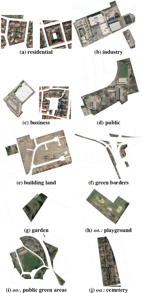
We distinguish nine land cover classes: building (build.), sealed area (seal.), bare soil (soil), grass, tree, water, rails, car, others. The number of land use classes varies during the experimental evaluation. The land use classes are refined step-wise in a hierarchical manner, following the hierarchical structure of most object catalogues for land use databases. In our case, we derive the class structure from the object catalogue of ALKIS® (AdV, 2008). At the coarsest semantic level, this object catalogue differentiates four main categories of land use, i.e. settlement, traffic, vegetation and water body. These categories are split into different object types, which are again subdivided into different object functions. In total, this leads to a very detailed description of land use in this specific object catalogue by approximately 190 different classes. Table 1 shows the land use classes which we try to distinguish in our experiments, giving also the number of samples of each class for both test data sets. In the coarsest semantic level, the main land use groups of the object catalogue are extended to six classes by dividing the class vegetation into agriculture and forest as well as by adding the class others, which mainly includes object types such as public gardens, playgrounds, etc., that belong to the main category settlement in ALKIS®. Fig. 1 shows examples for some of the subcategories of the main categories settlement and others.
The analysis of the separability of the subcategories for each of the main categories in Table 1 are described in Section 4.2. In Section 4.3 we investigate if the use of additional, more sophisticated features leads to improved results. In Section 4.4 the impact of using spatial context in the classification process is assessed.
4.2 Step-wise refinement of the class structure
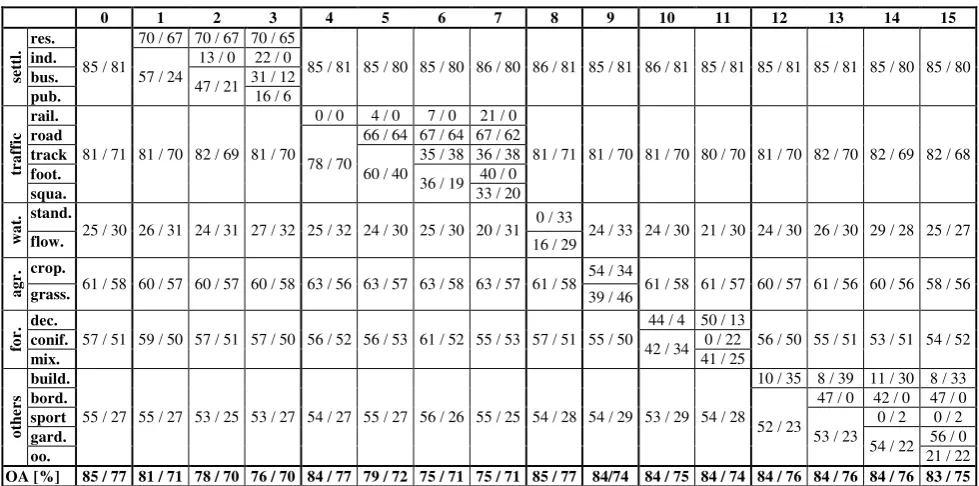
in the previous step. The quality values for each class (as a trade-off between completeness and correctness) and the overall accuracy of the classification results are shown in Table 2. We start with distinguishing only the six main categories described in Section 4.1 (experiment 0 in Table 2). After that, we refine the class structure for one main category after the other, leaving the others at the coarsest semantic level. The refinement is carried out in a hierarchical manner. For instance, the main category settlement is split into two subcategories first (res. vs. the union of ind., bus. and pub.; cf. experiment 1 in Table 2), afterwards we distinguish three (res., ind., union of bus. and pub.; cf. experiment 2 in Table 2), and finally four subcategories (cf. experiment 3 in Table 2). This strategy is pursued for all main categories.
Category Subcategory Abb. Description HM SL
settlement (settl.)
residential res. detached houses,
densely built-up areas 503 899
industry ind. production industry,
craft 90 32
business bus. trade, other services 181 119
public pub.
community facilities, e.g. school, administration
193 252
traffic
railway rail. 23 2
road road 482 666
track track 284 428
footpath foot. 372 1
public square squa. e.g. market, parking lot 89 166 water body
(wat.)
standing wat. stand. e.g. sea, lake, pond 4 91 flowing wat. flow. e.g.river, stream, trench 53 90 agriculture
(agr.)
cropland crop. 64 260
grassland grass. 89 426
forest (for.)
deciduous for. dec. 25 98
coniferous for. conif. 4 41
mixed forest mix. 60 135
others (oth.)
building land build. 34 64
green borders bord. 185 36
sport areas sport 6 26
garden gard. 170 8
others oo. e.g. playgrounds,
public green areas 131 354
Table 1.Hierarchical class structure and number of samples for the test areas “Hameln” (HM) and “Schleswig” (SL). Abb.:
abbreviation used in the remaining text.
Looking at the results in Table 2, the first thing to be observed is that the overall accuracy obtained in the test area Hameln is consistently higher than in the test area Schleswig (e.g. by 8% if only the main categories are distinguished). This is mainly caused by different characteristics of the test areas and acquisition dates of the aerial images. For both test sites, the overall accuracy decreases slightly in the refinement process. The lowest values are about 10% below the level achieved for the main categories and are generally achieved for the finest class structure. Table 2 shows that in the refinement process, the level of quality remains nearly unchanged for the classes that are not refined, but it is decreased dramatically for some subcategories as the class structure is refined. Thus, the decrease in overall accuracy which can be observed during refinement is mainly caused by an increase of wrong assignments between classes within the currently refined main category. This process does not lead to a significant increase of wrong assignments among the main categories.
4.2.1 Settlement: For the category settlement, it is possible to separate the land use class residential from the other built-up land use classes in the test area Hameln with high quality:
69.9% for residential and 56.8% for the group of other built-up land use classes. With a further refinement of the second group into industry, business and public, the quality decreases significantly; i.e. in the finest level of detail 22.2% for industry, 31.1% for business and 16.3% for public land use. The loss in quality results mainly from a confusion between the subcategories. Similarities in the appearance of these objects lead to wrong decisions. In Fig. 1, showing samples of each subcategory of settlement, the problem of similar appearance becomes obvious. Even for a human operator it is impossible to distinguish e.g. the classes residential and business, especially in densely built-up areas (cf. Fig. 1 (a, right) and (c, right)). Furthermore, the building structure (large, flat buildings) as well as the land cover components (for the most part sealed area and buildings) in business and industrial areas are quite similar (cf. Fig. 1 (b) and (c, left)). These two classes only describe different but closely related business purposes, which makes a distinction based on remote sensing data impossible.
(a) residential (b) industry
(c) business (d) public
(e) building land (f) green borders
(g) garden (h) oo.: playground
(i) oo:. public green areas (j) oo.: cemetery
The low quality of 16.3% for the land use public results from its heterogeneous appearance, which is reflected by wrong assignments to the classes residential, traffic and business in nearly equal shares. This class contains schools and administrative buildings mainly characterised by large buildings and green areas (cf. Fig.1 (d)) as well as power distribution areas, which are composed of very small buildings on small pieces of land typically located close to residential areas. In the test area Schleswig, even the discrimination of residential from non-residential classes is challenging, which is mainly caused by the characteristics of the test area. Many objects of these classes have a more similar appearance with respect to e.g. building structure than in the test area Hameln. For instance, industrial areas are composed of smaller buildings with gabled roofs and vegetated as well as sealed areas instead of large, flat buildings and a high degree of sealing, which makes them more similar to all other settlement classes.
4.2.2 Traffic: For the category traffic, the best accuracy in a fine-grained class structure can be achieved for the class road with a quality value of 66.5% (Hameln) and 61.9% (Schleswig). The discrimination of road is facilitated by its uniform appearance (elongated shape, dominated by sealed area). In contrast, the class track typically also has an elongated shape, but differs concerning its material (asphalt, gravel, grass). This leads to a lower quality of 35.9% (Hameln) and 37.7% (Schleswig). In Hameln, the class railway can be discriminated better from other classes if a very detailed class structure is distinguished, whereas in the first step of the refinement, not a single railway object is detected correctly. Most of the railway objects are misclassified as roads. The number of correctly classified objects increases in each step of refinement. Nevertheless, in the finest class structure a quality of only 20.7% is achieved, which results from a low completeness value of 20.7% in spite of a high correctness value of 100%. In Schleswig, railway cannot be differentiated from the other subcategories at all. The particularly low quality values for railway and (in Schleswig) footpath also results from the low number of samples (less than 25 in the whole test area), so that
these results are hardly representative. For the subcategory square a quality of 33.3% (Hameln) and 20.3% (Schleswig) can be achieved.
4.2.3 Water body: In Hameln, a more detailed distinction of the category water body fails due to the low number of training samples, especially for standing water body. As there is no difference in the spectral characteristics of these classes, the discrimination can only be based on the shape of the land use objects (elongated shape for flowing water body and a more compact shape for standing water body). The number of samples available for training in this test area is not sufficient to train the classifier appropriately, especially as these samples belong to different kinds of standing water bodies which differ again in their shape, such as lake and pond. Due to a higher number of training samples in the second test area, a better accuracy is achieved with a quality of 33.3% for flowing water body and 29.1% for standing water body. Nevertheless, objects are wrongly assigned to the other class within the category.
4.2.4 Agriculture: The extent to which cropland can be distinguished from grassland depends on the vegetation coverage in the cultivation cycle. In spring, cropland is mostly covered by soil, which enables a clear distinction of grassland. Later in the year, the vegetation grows, so that the spectral appearance of cropland becomes more and more similar to grassland. In this case, a regular pattern of tractor tracks is the only evidence for the class cropland. As the aerial images of Hameln were captured in spring, there are favourable conditions for correctly classifying cropland objects, so that a correctness of 73.9% and completeness of 66.2% are achieved. The classification of grassland is more challenging due to similarities with urban green areas, such as parks and building land. This results in a lower correctness of 53.5% and a lower completeness of 59.8%. The discrimination of cropland and grassland is much more challenging in Schleswig due to fact that the aerial images were acquired in summer. At this time of the year, croplands are hard to distinguish from grassland, leading to a lower quality value for cropland of 33.5%.
0 1 2 3 4 5 6 7 8 9 10 11 12 13 14 15
Table 2. Quality measures [%] and overall accuracy (last row; OA) [%] for the land use classes defined in Table 1 obtained by applying our classification approach to hierarchically refined class structures for the test areas Hameln (first entry in each field) and Schleswig (second entry). The first row contains an index for the experiment. In experiments 1-3, more and more subcategories for
4.2.5 Forest: In Hameln, the category forest can be subdivided into deciduous and mixed forest (including coniferous forest), while achieving quality values of above 40%. The correctness of the class deciduous forest is quite high (88.2%), but the quality measure is worse due to a low completeness of 46.9%. In contrast, a higher completeness of 64.9% is achieved for the class mixed forest, but this goes along with a lower correctness of 54.5%, thus, leading to a quite similar quality measure. The discrimination of the class coniferous tree fails due to the small number of training samples for this class. As the aerial images of Schleswig were acquired when the trees were covered with leaves, a discrimination of different forest types is difficult.
4.2.6 Others: The refinement of the category others shows that only the classes garden and green borders can be discriminated appropriately in the test area Hameln, which are the classes with the most training samples in this test area. This gives yet another indication for the dependency between the classification accuracy and the number of training samples. In Schleswig only a low number of green borders and gardens are contained.
4.2.7 Discussion: The quality values obtained for the two test sites show that there are three main impact factors restricting the maximum level of semantic resolution that can be achieved. First, some classes are so similar in appearance that they cannot be differentiated, which, however, may vary with regional characteristics of the area under investigation (cf. Section 4.2.1). Second, the characteristics of the sensor data, in particular the acquisition date, has a major impact, especially for the discrimination of classes related to vegetation. Finally, and not surprisingly, the number and representativeness of training samples is a limiting factor. Land use objects may cover a large area, so that one ends up with very few training samples even if classifying a large area (the test area Schleswig contains 30,0002 pixels). Taking the Hameln data as a reference due to their more appropriate acquisition date and selecting classes achieving a quality larger than 30%, we can distinguish a maximum level of semantic resolution of nine classes: residential, non-residential (non-res.), route (includes rail., road, track and foot.), square, cropland, grassland, deciduous forest, mixed forest and urban green areas (urb. gr.). In the subsequent sections we distinguish these nine classes and water body, which is chosen as a main category in spite of low quality values.
4.3 Feature Importance
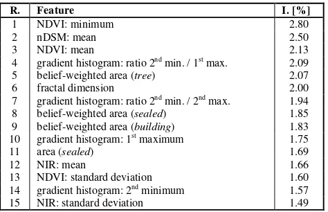
To investigate the impact of the extracted features on the classification result, we analyse the relevance of each feature based on the permutation importance measure of the RF classifier (Breiman, 2001). Table 3 shows the importance measures for the 15 most important features used for estimating the association potential in land use classification. This list contains features of all major categories (spectral, three-dimensional, geometrical, contextual). In particular, four of the 15 most important features are contextual ones. All of them are spatial metrics, namely the belief-weighted proportion of the area of the land cover classes building, sealed area and tree within a land use object and the percentage of the area covered by the land cover class sealed area. Thus, contextual features encoding the composition of land cover elements within a land use object have proven to be of high relevance for land use classification, whereas the graph-based measures derived from the adjacency-event-matrix as well as the features describing the distribution of land cover elements within a land use object are of less importance. Based on the feature importance measure, we select the 40 most important features for land cover and land use classification for the final experiments in Section 4.4.
R. Feature I. [%]
1 NDVI: minimum 2.80
2 nDSM: mean 2.50
3 NDVI: mean 2.13
4 gradient histogram: ratio 2nd min. / 1st max. 2.09
5 belief-weighted area (tree) 2.07
6 fractal dimension 2.00
7 gradient histogram: ratio 2nd min. / 2nd max. 1.94
8 belief-weighted area (sealed) 1.85
9 belief-weighted area (building) 1.83
10 gradient histogram: 1st maximum 1.75
11 area (sealed) 1.69
12 NIR: mean 1.66
13 NDVI: standard deviation 1.60
14 gradient histogram: 2nd minimum 1.57
15 NIR: standard deviation 1.49
Table. 3. The 15 most important features for the classification of the association potential in the land use layer in Hameln, ranked
by their feature importance values (I.); R.: rank.
4.4 Classification results
Table 4 shows the results obtained for the contextual classification of the test data from Hameln and Schleswig using the features selected in the way described in Section 4.3 and differentiating the ten classes identified in Section 4.2.7. For a comparison, we also included the results of an independent RF-based classification (without considering context) for Hameln.
HM - RF-class. HM – CRFcontext SL – CRFcontext
Table 4.Completeness (comp.), correctness (corr.) [%], overall accuracy (OA) [%], and kappa index [%] for the ten land use
classes defined in Section 4.2.7, obtained by applying a RF-classifier (RF-class.) and the contextual classification approach (CRFcontext) to the test areas Hameln (HM) and Schleswig (SL).
The consideration of context leads to an improved classification accuracy for certain classes, i.e. non-residential, deciduous forest and urban green areas. The completeness increases for the classes grassland and mixed forest, which goes along with a decrease in correctness. For the class residential, the correctness increases significantly, while the completeness decreases. The correctness of the class square and the completeness and correctness of the classes water body and cropland decrease. In general, the accuracies for the test area Schleswig are much lower for reasons already discussed in Sec. 4.2.
more than 10% compared to the maximum level of refinement of this category (experiment 7 in Table 2), which is mainly caused by wrong assignments of these objects to route. The class square suffers from the aggregation of all other traffic classes to one class, which leads to a higher variability of that class (route). For the class water body, the completeness and the correctness decrease due to an increase of the number of objects erroneously classified as route or others. However, for most of the other classes (e.g. for residential and non-residential), the quality remains nearly constant. Basically, discriminating the set of classes identified in Section 4.2.7 seems to be possible.
5. CONCLUSION
We have investigated the maximum level of semantic resolution that can be achieved by an approach for the contextual classification of aerial imagery to determine land cover and land use simultaneously (Albert et al., 2015). Our experiments show that a semantic resolution of ten classes still delivers acceptable results. The maximum level of semantic resolution that can be achieved is mainly restricted by a similar appearance of classes, the characteristics of the sensor data and the number and representativeness of training samples in the area under investigation. Furthermore, our experiments confirm that the incorporation of contextual knowledge, especially in the form of contextual features, is beneficial for land use classification.
Nevertheless, further work is required in order to improve the classification results. Remaining problems may result from the fact that for some classes we currently have only a small number of training samples, thus, not all classes are properly and equally represented in the training data. Therefore, we want to apply our approach on more test areas with different characteristics and more training data, especially for currently underrepresented classes. Furthermore, the method investigated here is only the first step of a scheme for updating a geospatial database. Currently, the geometric delineation of the geospatial objects is assumed to be correct; in the future, we aim to infer changes of the geometric outlines of objects automatically, e.g. by splitting and merging objects.
ACKNOWLEDGEMENT
We thank the Landesamt für Geoinformation und Landesvermessung Niedersachsen (LGLN) and the Landesamt für Vermessung und Geoinformation Schleswig Holstein (LVermGeo) for providing the test data and for their support of this project.
REFERENCES
Achanta, R., Shaji, A., Smith, K., Lucchi, A., Fua, P. & Susstrunk, S., 2012. SLIC superpixels compared to state-of-the-art superpixel methods. IEEE Transactions on Pattern Analysis and Machine Intelligence 34(11), pp. 2274-2282.
Albert, L., Rottensteiner, F., Heipke, C., 2014. Land use classification using Conditional Random Fields for the verification of geospatial databases. In: ISPRS Annals of Photogrammetry, Remote Sensing and Spatial Information Sciences, vol. II-4, pp. 1-7.
Albert, L., Rottensteiner, F., Heipke, C., 2015. An iterative inference procedure applying Conditional Random Fields for simultaneous classification of land cover and land use. ISPRS
Annals of Photogrammetry, Remote Sensing and Spatial Information Sciences, vol. II-3/W5, pp. 369-376.
Arbeitsgemeinschaft der Vermessungsverwaltungen der Länder der Bundesrepublik Deutschland (AdV), 2008. ALKIS® -Objektartenkatalog 6.0. Available online (visited 07/04/2016):
http://www.adv-online.de/AAA-Modell/Dokumente-der-GeoInfoDok/
Banzhaf, E., Hofer, R., 2008. Monitoring urban structure types as spatial indicators with cir aerial photographs for a more effective urban environmental management. IEEE Journal of Selected Topics in Applied Earth Observations and Remote Sensing 1(2), pp.129-138.
Barnsley, M. J., Barr, S. L., 1997. Distinguishing urban land-use categories in fine spatial resolution land-cover data using a graph-based, structural pattern recognition system. Computers, Environment and Urban Systems 21(3), pp.209-225.
Barr, S., Barnsley, M., 1997. A region-based, graph-theoretic data model for the inference of second-order thematic information from remotely-sensed images. International Journal of Geographical Information Science 11(6), pp.555-576.
Breiman, L., 2001. Random Forests. Machine Learning 45, pp.5-32.
Frey, B. and MacKay, D., 1998. A revolution: Belief propagation in graphs with cycles. In: Advances in Neural Information Processing Systems, vol. 10, pp.479-485.
Haralick, R.M., Shanmugan, K., Dinstein, I., 1973. Texture features for image classification. IEEE Transactions on Systems, Man and Cybernetics 3, pp.610-621.
Helmholz, P., Rottensteiner, F., Heipke, C., 2014. Semi-automatic verification of cropland and grassland using very high resolution mono-temporal satellite images. ISPRS Journal of Photogrammetry and Remote Sensing 97, pp.204-218.
Hermosilla, T., Ruiz, L.A., Recio, J.A., Cambra-López, 2012. Assessing contextual descriptive features for plot-based classification of urban areas. Landscape and Urban Planning 106(1), pp.124-137.
Kumar, S., Hebert, M., 2006. Discriminative Random Fields. International Journal of Computer Vision 68(2), pp.179–201.
Novack, T., Stilla, U., 2015. Discrimination of urban settlement types based on space-borne sar datasets and a conditional random fields model. ISPRS Annals, vol.1, pp.143-148.
Rutzinger, M., Rottensteiner, F., Pfeifer, N., 2009. A comparison of evaluation techniques for building extraction from airborne laser scanning. IEEE Journal of Selected Topics in Applied Earth Observations and Remote Sensing 2(1), pp.11-20.