ALTERNATIVE METHODOLOGIES FOR THE ESTIMATION OF LOCAL POINT
DENSITY INDEX: MOVING TOWARDS ADAPTIVE LIDAR DATA PROCESSING
Z. Lari, A. Habib
Dept. of Geomatic Engineering, University of Calgary, 2500 University Drive N.W., Calgary, AB, T2N1N4, Canada
(zlari, ahabib)@ucalgary.ca
Commission III, WG II/2
KEY WORDS: LIDAR, Point cloud, Processing, Estimation, Quality, Analysis
ABSTRACT:
Over the past few years, LiDAR systems have been established as a leading technology for the acquisition of high density point clouds over physical surfaces. These point clouds will be processed for the extraction of geo-spatial information. Local point density is one of the most important properties of the point cloud that highly affects the performance of data processing techniques and the quality of extracted information from these data. Therefore, it is necessary to define a standard methodology for the estimation of local point density indices to be considered for the precise processing of LiDAR data. Current definitions of local point density indices, which only consider the 2D neighbourhood of individual points, are not appropriate for 3D LiDAR data and cannot be applied for laser scans from different platforms. In order to resolve the drawbacks of these methods, this paper proposes several approaches for the estimation of the local point density index which take the 3D relationship among the points and the physical properties of the surfaces they belong to into account. In the simplest approach, an approximate value of the local point density for each point is defined while considering the 3D relationship among the points. In the other approaches, the local point density is estimated by considering the 3D neighbourhood of the point in question and the physical properties of the surface which encloses this point. The physical properties of the surfaces enclosing the LiDAR points are assessed through eigen-value analysis of the 3D neighbourhood of individual points and adaptive cylinder methods. This paper will discuss these approaches and highlight their impact on various LiDAR data processing activities (i.e., neighbourhood definition, region growing, segmentation, boundary detection, and classification). Experimental results from airborne and terrestrial LiDAR data verify the efficacy of considering local point density variation for precise LiDAR data processing.
1. INTRODUCTION
In recent years, Light Detection and Ranging (LiDAR) systems are being extensively utilized for rapid collection of high density 3D point clouds. These point clouds provide accurate 3D data for different applications such as terrain mapping (Elmqvist et al., 2001), transportation planning (Uddin and Al-Turk, 2001), 3D city modeling (Kim et al., 2008), heritage documentation (Patias et al., 2008), and forest parameter estimation (Danilin et al., 2004). The collected data should be processed to extract useful information for the aforementioned applications. The internal properties of LiDAR point cloud and the performance of processing techniques highly affect the validity of extracted information. Point density is an important characteristic of LiDAR data that should be considered during the various processing activities (e.g., neighbourhood definition, classification, segmentation, feature extraction, and object recognition).
The majority of existing data processing techniques assumes that the LIDAR point cloud has a uniform point density. However, the collected data might show variations in the point density due to irregular movements of the acquisition platform, variations in the scattering properties of the mapped surface, number of overlapping strips, and incorporation of terrestrial laser scanning systems (Vosselman and Mass, 2010). Therefore, data processing techniques should consider possible variations in the point density within the datasets in question. This ability will assure the flexibility of these techniques in dealing with datasets captured by different platforms and/or from different sources. The effective consideration of these variations is
dependent on providing standard approaches for the estimation of local point density indices.
So far, only a few applicable methods have been presented for the determination of local point density indices. The most commonly used method for the estimation of local point density is the “box-counting method” proposed by County (2003). In this method, the LiDAR points are firstly projected onto a 2D space. Then, the defined 2D space is rasterized using a grid with a predefined cell size. The local point density index for the points within each cell is then determined as the total number of the projected points in that cell normalized by the cell area. The main disadvantage of this method is that the estimated local point density values are dependent on the size of the cells and their placement within the projected data. Since there is no standard for the determination of the appropriate cell size and its placement within a LiDAR data, different density values may be estimated for the same points in a LiDAR dataset (Raber et al., 2007).
In order to estimate unique local point values for individual LiDAR points, Shih and Huang (2006) proposed a TIN-based method. In this method, the point cloud is firstly triangulated using an advanced Delaunay triangulation technique (Isenburg, 2006) to produce a TIN. Then, a Voronoi Diagram is constructed utilizing the generated TIN structure. The local point density index for each point is then estimated by inversing the area of the Voronoi polygon assigned to that point. The presented approaches for the local point density estimation only consider the 2D distribution of the point cloud. Therefore, they are only valid when dealing with point cloud acquired by an International Archives of the Photogrammetry, Remote Sensing and Spatial Information Sciences, Volume XXXIX-B3, 2012
airborne system over relatively flat horizontal terrain and cannot be applied for terrestrial laser scans.
The shortcomings of the aforementioned approaches mandate the development of alternative methods for the local point density estimation. In this paper, new approaches are proposed for the estimation of local point density indices. These approaches aim to derive unique/accurate point density values for individual LiDAR points while considering the 3D relationships among them and physical properties of the surfaces they belong to. Furthermore, the implication of considering the varying point density in different LiDAR data processing activities will be highlighted in this paper.
The paper starts with the introduction of the proposed approaches for local point density estimation. In the following section, the impact of considering the local point density indices on some of LiDAR data processing activities is pointed out and discussed. In the next section, the performance of the proposed methods for local point density estimation and the impact of considering these local indices on LiDAR data processing results are evaluated through experimental results using airborne and terrestrial LiDAR datasets. Finally, concluding remarks and recommendations for future research work will be presented.
2. METHODOLOGY
This section introduces alternative methodologies for the estimation of local point density indices. These methods try to overcome the shortcomings of previous approaches by considering the 3D relationships among the points and the physical properties of the surfaces enclosing the individual points.
In the following subsections, the detailed explanation of these approaches is presented and their advantages and disadvantages are pointed out.
2.1 Approximate Method
In this method, the local point density index for each point is computed while only considering the distribution of the points within its spherical neighbourhood. This neighbourhood is defined to include n-neighbours of the point in question ( Figure 1), where n is a pre-specified number of neighbouring points.
Figure 1. 3D neighbourhood of the point in question (POI)
For a given LiDAR point, the local point density (LPD) is question with a radius (rn) that is equivalent to the distance from this point to its nth-nearest neighbour.
This approach provides a unique estimate of the local point density for all the points in a LIDAR dataset in a fast and simple manner. Therefore, this approach can be efficiently utilized for
in-flight quality assessment of the collected LiDAR point cloud. However, it suffers from the following shortcomings:
− It does not consider the physical properties of the surface which the point in question and its neighbouring points belong to.
− It assumes a uniform distribution of the points in the 3D space defined by the point in question and its neighbouring points.
2.2 Eigen-value Analysis of the Dispersion of Neighbouring
Points
In order to resolve the first drawback of previous method, this approach estimates the local point density only when the point in question and its neighbouring points define a planar region. In this method, a spherical neighbourhood of the point in question is initially defined. This neighbourhood encloses the n-nearest neighbours of the point in question, where n is the number of points needed for reliable plane definition while considering the possibility of having some outliers. The planarity of the established 3D neighbourhood is investigated using the eigen-value analysis of the dispersion matrix of the (n+1) points within the spherical neighbourhood of the point in question relative to their centroid (C) (Figure 2).
Figure 2: Dispersion of the points within the established 3D neighbourhood relative to their centroid
This dispersion matrix (C1) is computed as follows (Pauly et al., 2002):
The eigen-value decomposition of the dispersion matrix (C1) results in three eigen values ( 1, 2, 3). For planar neighbourhoods, one of the eigen values will be quite small when compared to the other two eigen values. This eigen value corresponds to the eigen vector which is perpendicular to the plane passing through those points. Once the planarity of the established neighbourhood is confirmed, the local point density is estimated in the same way as the approximate approach.This approach overcomes the first drawback of the approximate method by considering the planarity of the surface enclosing the point in question. However, it still assumes a uniform distribution of the points within the established 3D neighbourhood. This approach also has the following shortcomings:
− It does not check whether the point in question belongs to the planar surface passing through the neighbouring points or not.
− When the majority of the points in the established 3D neighbourhood are coplanar, non-coplanar points are considered in the estimation of the local point density. To resolve these problems, the planarity of the established 3D neighbourhood is checked using the eigen-value analysis of the dispersion matrix of the neighbouring points within the International Archives of the Photogrammetry, Remote Sensing and Spatial Information Sciences, Volume XXXIX-B3, 2012
established 3D neighbourhood relative to the point in question (POI) (Figure 3).
Figure 3: Dispersion of the points within the established 3D neighbourhood relative to the point in question In this case, the dispersion matrix (C2) is derived as follows:
question belongs to the local plane through this neighbourhood. Once the planarity of established neighbourhood is checked, the local point density index is estimated in the same way as the approximate method.
Despite considering if the point question belongs to planar neighbourhood or not, this approach is still subjected to the inclusion of non-coplanar points within established 3D neighbourhood for local point density estimation.
spherical neighbourhoods is investigated by defining a cylinder whose axis orientation is adaptively changing to be aligned along the normal to the plane through the majority of the points in the defined neighbourhood (Figure 4). This axis is derived using an iterative plane fitting procedure where the points are assigned weights that are inversely proportional to their normal distances from the derived plane in the previous iteration.The cylinder diameter is equivalent to the distance between the point in question and its nth-nearest neighbouring point within the defined neighbourhood. The height of the defined cylinder is determined based on the expected noise level in the point cloud.
Figure 4: Adaptive cylinder neighbourhood In this approach, the local point density index is estimated only when the majority of the points within the established spherical neighbourhood, together with the point in question, are included in the defined cylinder. The local point density index is then computed as follows:
Where k is the number of the points within the defined cylinder and rn is the distance between the point in question and its nth -nearest neighbouring point in the spherical neighbourhood. This method estimates the local point density only by utilizing the points inside the adaptive cylinder. This resolves the drawback of the eigen-value analysis methods by removing the points which do not belong to the planar neighbourhood. The only shortcoming of this method is assuming a uniform point distribution within the adaptive cylinder.
3. THE IMPACT OF CONSIDERING LOCAL POINT
DENSITY INDICES ON LIDAR DATA PROCESSING
As mentioned earlier, the consideration of local point density indices will improve the LiDAR data processing results to a great extent. In this section, some of the processing activities which are highly affected by local point density variations are highlighted and the impact of incorporating estimated local density values in these activities are discussed.
3.1 Neighbourhood Definition
Neighbourhood definition is the primary step of LiDAR data processing. This definition is a rule that determines the neighbours of each point, and as a result has a great impact on the reliability of different processing activities’ results. Different neighbourhood definitions are presently being used for LiDAR data. However, none of them consider the local variations in the LiDAR point density. This inconsideration leads to the exclusion of required neighbouring points and inclusion of the points that should not be considered for the derivation of processing parameters (e.g, segmentation attributes). In order to define meaningful neighbourhoods for individual LiDAR points, while considering the characteristics of their associated surfaces, the computed local point density indices should be considered. In this case, when the local point density is low, the size of the defined neighbourhood will be increased to include the needed number of points for the derivation of processing parameters.
3.2 Region Growing
Region growing is recognized as one of the spatial-domain LiDAR data segmentation approaches. In this approach, the neighbouring LiDAR points that fulfil a homogeneity criterion (e.g., planarity or smoothness of the surface) will be segmented in one group (Besl and Jain, 1988). The conventional criterion for the determination of neighbouring points, in this process, is a fixed 3D distance. However, when the local point density is not uniform within a LiDAR dataset, considering a fixed neighbourhood radius may result in inaccurate segmentation results. In order to define adaptive neighbourhoods of the seed points for region growing, the local point density index in the seed point location should be incorporated in the definition of the neighbourhood radius.
3.3 Derivation of Attributes for Parameter-Domain
Segmentation Approaches
The performance of the parameter-domain segmentation methods depends on the computed attributes for individual laser points. In most of these approaches, the segmentation attributes are derived based on the parameters of the fitted plane through the neighbouring points within the defined neighbourhood for each point. The quality of plane fitting process is ensured by providing the needed number of points for the plane definition. Therefore, the size of established neighbourhood should be made flexible with International Archives of the Photogrammetry, Remote Sensing and Spatial Information Sciences, Volume XXXIX-B3, 2012
local point density variations to include the required number of points for reliable plane definition.
3.4 Boundary Detection
The major drawback of parameter-domain segmentation techniques is that the spatial connectivity of points belonging to each segment is not considered. Therefore, the points belonging to coplanar but spatially disconnected planes will be segmented into the same group. To resolve such ambiguity, a neighborhood analysis is conducted through boundary detection of the clustered points. The process of searching for each boundary point is carried out in the local neighbourhood of the previous boundary point. In order to define adaptive neighbourhoods for sequentially finding the boundary points, the estimated local point density indices should be taken into consideration.
3.5 Terrain/Off-terrain Classification
In order to classify the clusters of LiDAR points into those belonging to terrain or off-terrain objects, the discontinuity measures between adjacent clusters should be considered. The adjacency relationship between these clusters is defined by analyzing the neighbourhoods of each cluster’s boundary points. For all the points in the boundary of each cluster, there exist neighbourhoods which include the points belonging to its adjacent clusters. In order to define adaptive neighbourhoods which include the points belonging to adjacent segments, the local point density index at each point’s location should be considered.
4. EXPERIMENTAL RESULTS
In this section, the performance of the newly developed methods for the estimation of the local point density indices and the impact of considering them on the quality of LiDAR data segmentation results will be investigated by conducting experiments using airborne and terrestrial LiDAR datasets.
4.1 Airborne LiDAR Data
The utilized airborne LiDAR dataset for this experiment (Figure 7.a) has been collected over an urban area in Switzerland with the Scan2Map mapping system. This dataset exhibits significant local point density variations (estimated by the approximate method) as shown in Figure 7.b. The results of the planarity check for the individual points using the eigen-value analysis and adaptive cylinder methods are presented in figures 7.c and 7.e, respectively. Once the planarity of individual points was checked and local point density indices were calculated, the point density maps for the points belonging to planar surfaces are generated using estimated local point density indices (figures 7.d and 7.f).
(a) (b)
(c) (d)
(e) (f)
Figure 7. Airborne LiDAR dataset: (a) original LiDAR data, (b) generated point density map using the approximate method, (c) planarity check result using the eigen-value analysis relative to the point in question, (d) generated point density map based
on eigen-value analysis relative to the point in question, (e) planarity check result using the adaptive cylinder method, and (f) generated point density map based on adaptive cylinder
method
To verify the importance of the processing of LiDAR data while considering the estimated local point density indices, the provided airborne datasets is processed using an adaptive segmentation approach (Lari et al., 2011). The segmentation process is carried out with and without considering local point density variations. Figure 8.a shows the result of the airborne LiDAR data segmentation without considering local point density variations while Figure 8.b shows the result of the segmentation of the same data considering the local point density variations. Qualitative evaluation of the derived segmentation results through visual inspection of Figures 8.a and 8.b shows that considering the local point density indices avoids some problems in the segmentation results, the most visible one is the over-segmentation problem – as highlighted within the red rectangles.
(a) (b)
Figure 8. Airborne LiDAR dataset segmentation results: (a) without considering local point density variations and
(b) considering local point density variations
4.2 Terrestrial LiDAR Data
The terrestrial LiDAR dataset (Figure 9.a) has been obtained from a building façade in the University of Calgary campus 28.05 Pnts/m2
0.03 Pnts/m2
26.24 Pnts/m2
0.004 Pnts/m2 Planar
Non-Planar
Planar Non-Planar
28.89 Pnts/m2
0.12 Pnts/m2
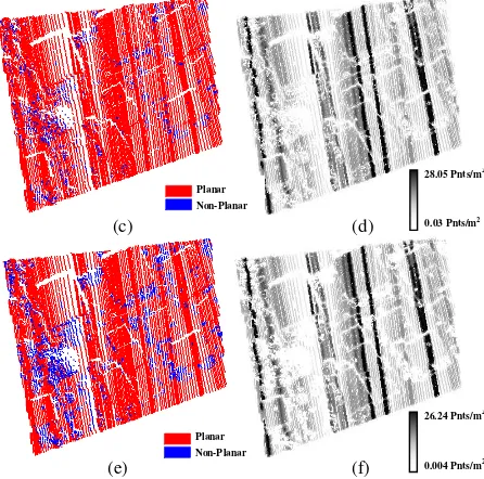
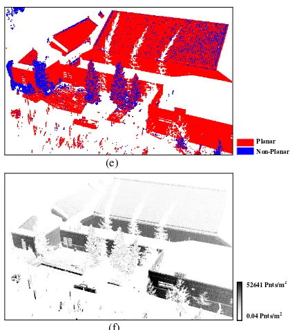
using Trimble GS200 3D laser scanner. The local point density map of this dataset, estimated by the approximate method, is shown in Figure 9.b. The results of the planarity check for the individual points using the eigen-value analysis and adaptive cylinder methods are presented in Figures 9.c and 9.e, respectively. The point density maps for the points belonging to planar surfaces are then generated using estimated local point density indices (Figures 9.d and 9.f).
(a)
(b)
(c)
(d)
(e)
(f)
Figure 9. Terrestrial LiDAR dataset: (a) original LiDAR data, (b) generated point density map using the approximate method, (c) planarity check result using the eigen-value analysis relative to the point in question, (d) generated point density map based
on eigen-value analysis relative to the point in question, (e) planarity check result using the adaptive cylinder method, and (f) generated point density map based on adaptive cylinder
method
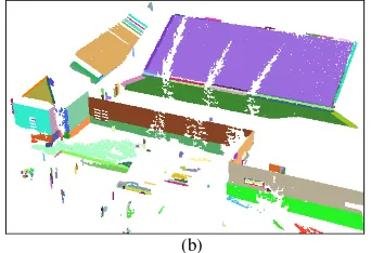
To assess the impact of considering the estimated local point density indices on the quality of terrestrial LiDAR data segmentation results, this dataset is segmented using the cited segmentation approach. The segmentation process is performed with and without considering local point density variations. Figure 10.a shows the result of the terrestrial LiDAR data segmentation without considering local point density variations while Figure 10.b shows the result of the segmentation of the same data while considering the local point density variations. The comparison of the derived segmentation results with and without considering the estimated local point indices demonstrates that considering the local point density indices avoids the over-segmentation problems in the segmentation results.
(a) 55919 Pnts/m2
0.45 Pnts/m2
Planar Non-Planar
Planar Non-Planar
53220 Pnts/m2
0.11 Pnts/m2
52641 Pnts/m2
0.04 Pnts/m2 International Archives of the Photogrammetry, Remote Sensing and Spatial Information Sciences, Volume XXXIX-B3, 2012
(b)
Figure 10. Terrestrial LiDAR dataset segmentation results: (a) without considering local point density variations and
(b) considering local point density variations
5. CONCLUSIONS AND RECOMMENDATIONS FOR
FUTURE RESEARCH WORK
In this paper, alternative methodologies have been presented for the estimation of local point density indices. These methods try to overcome the shortcomings of available methods by considering the 3D relationships among LiDAR points and physical properties of the enclosing surfaces. In the simplest approach, the local point density index is estimated while considering a pre-defined number of neighbouring points to the point in question in 3D space normalized by by the area of the circle that comprises these neighbouring points. Although this approach is simple and computationally efficient, it does not take the physical properties of the surfaces enclosing the individual points into account. In the other approaches, the planarity of the surfaces enclosing the LiDAR points is firstly checked through eigen-value analysis or adaptive cylinder definition. Then, the local point density indices are estimated for the points belonging to planar surfaces. The main advantage of the eigen-value analysis over the adaptive cylinder definition is the efficient computation. However, this approach is not able to filter out the neighbouring points which do not belong to the planar neighbourhood of the point in question prior to the estimation of the local point density index. In spite of its computational burden, the adaptive cylinder definition technique can provide more accurate point density estimations by filtering out the outliers that do not belong to the planar neighbourhoods before the computation of the local point density indices. The other advantage of the this method is directly providing the segmentation attributes through the parameters of the best fitting plane through the points within the defined adaptive cylinder.
In order to demonstrate the impact of considering the estimated local point densities on the quality of LiDAR data processing, different cases have been discussed in which incorporating these indices leads to major improvements in the derived results. Future research work will focus on the quantitative evaluation of LiDAR data processing outcome (i.e., boundary detection, segmentation and classification) while considering the local point density variations and comparative analysis of these results with the results from other processing techniques.
ACKNOWLEDGEMENTS
This work was supported by the Canadian GEOmatics for Informed DEcisions (GEOIDE) Network of Centres of Excellence (NCE) (Project: PIV-SII72), the Natural Sciences and Engineering Research Council of Canada (Discovery and Strategic Project Grants), and TECTERRA. The authors would
also like to thank Dr. Jan Skaloud, EPFL (École Polytechnique Fédérale de Lausanne), Switzerland for providing the airborne LiDAR datasets.
REFERENCES
Besl P. J. and Jain, R. C., 1988. Segmentation through Variable-order Surface Fitting, IEEE Transactions on Pattern Analysis and Machine Intelligence, 10(2), pp.167-192.
County, K., 2003. LiDAR digital ground model point density,
http://www5.kingcounty.gov/sdc/raster/elevation/LiDAR_Dig ital_Ground_Model_Point_Density.html/, KGIS Center, Seattle, WA.
Danilin, I. M. and Medvedev, E. M., 2004. Forest inventory and biomass assessment by the use of airborne laser scanning method, example from Siberia, International Archives of Photogrammetry, Remote Sensing and Spatial Information Sciences, XXXVI (8/W2), pp. 139 – 144.
Elmqvist, M., Jungert, E., Persson, A., and Soderman, U., 2001. Terrain modeling and analysis using laser scanner data. International Archives of Photogrammetry and Remote Sensing, XXXIV-3/W4, pp. 219–227.
Isenburg, M., Liu, Y., Shewchuk, J., and Snoeyink, J., 2006. Streaming Computation of Delaunay Triangulations, Proceedings of ACM SIGGRAPH’06, New York, USA, pp. 1049-1056.
Kim, C., Habib, A., and Chang, Y., 2008. Automatic generation of digital building models for complex structures from LiDAR data, The International Archives of the Photogrammetry, Remote Sensing and Spatial Information Sciences, XXVII (B4), pp. 463 – 468.
Lari, Z., Habib A., and Kwak E., 2011. An Adaptive Approach for Segmentation of 3D Laser Point Cloud, International Archives of the Photogrammetry, Remote Sensing and Spatial Information Sciences, XXXVII-5/W12, Calgary, Canada.
Patias, P., Grussenmeyer, P., Hanke, K., 2008. Applications in cultural heritage documentation, Advances in Photogrammetry, Remote Sensing and Spatial Information Sciences, ISPRS Congress Book, 7, pp. 363–384.
Raber, G. T., Jensen, J. R., Hodgson, M. E., Tullis, J. A., Davis B. A., and Berglund, J., 2007. Impact of Lidar Nominal Post-spacing on DEM Accuracy and Flood Zone Delineation, Photogrammetric Engineering & Remote Sensing, 73(7), 793–804.
Shih, P.T, and C. M. Huang, 2006. Airborne Lidar Point Cloud Density Indices, American Geophysical Union, Fall Meeting 2006, abstract # G53C-0919.
Uddin, W. and Al-Turk, E., 2001. Airborne LIDAR digital terrain mapping for transportation infrastructure asset management, in Proceedings of Fifth International Conference on Managing Pavements, Seattle, Washington.
Vosselman, G. and Maas, H. G., 2010. Airborne and Terrestrial Laser Scanning. Whittles Publishing, Scotland, UK, 320 p.