```
DISCRETE EKF WITH PAIRWISE TIME CORRELATED MEASUREMENT NOISE FOR
IMAGE-AIDED INERTIAL INTEGRATED NAVIGATION
N.S. Gopaul, J.G. Wang, B. Hu (nileshgo, jgwang, baoxin)@yorku.ca
Department of Earth and Space Science and Engineering Faculty of Graduate Studies
York University, Toronto, Canada
Technical Commission II
KEY WORDS: Kalman filter, correlated noise, Cholesky factorization, shaping filter
ABSTRACT:
An image-aided inertial navigation implies that the errors of an inertial navigator are estimated via the Kalman filter using the aiding measurements derived from images. The standard Kalman filter runs under the assumption that the process noise vector and measurement noise vector are white, i.e. independent and normally distributed with zero means. However, this does not hold in the image-aided inertial navigation. In the image-aided inertial integrated navigation, the relative positions from optic-flow egomotion estimation or visual odometry are pairwise correlated in terms of time. It is well-known that the solution of the standard Kalman filter becomes suboptimal if the measurements are colored or correlated. Usually, a shaping filter is used to model time-correlated errors. However, the commonly used shaping filter assume that the measurement noise vector at epoch k is not only correlated with the one from epoch k1 but also with the ones before epoch k1. The shaping filter presented in this paper uses Cholesky factors under the assumption that the measurement noise vector is pairwise time-correlated i.e. the measurement noise are only correlated with the ones from previous epoch. Simulation results show that the new algorithm performs better than the existing algorithms and is optimal.
1. INTRODUCTION
The high demand for direct-georeferencing technique with low-cost multisensor integrated kinematic positioning and navigation systems in mobile mapping is continuously driving more research and development activities. The effective and sufficient utilization of images is among the most recent scientific and high-tech research tasks. In this particular field of mapping and imaging, we are engaging in the study of the image-aided inertial integrated navigation as the natural continuation of its past research in the multisensor integrated kinematic positioning and navigation (Kun et al, 2012). Inertial Navigation Systems (INS) are widely used in direct georeferencing systems and become the core component for the automation of the geospatial data acquisition. The solution accuracy of an INS alone deteriorates with time because the accelerometer and gyroscope measurements are contaminated with noise, biases, scaling errors and non-orthogonality errors. As a result, the errors on the INS position, velocity and attitude increase without bounds in free inertial mode. To inhibit or reduce the INS errors, supplementary sensors can be added to the system, for example Global Navigation Satellite Systems (GNSS) receivers, cameras, barometers and odometers to name a few (Aggarwal et al, 2010).
Cameras are inherently high-bandwidth and therefore have the potential for precise angular resolution. They are readily available and easy to be interfaced with (Miller et al, 2011). Furthermore it is more economic than the other self-contained electro-optical sensors such as laser ranging (LIDAR) (Shen et al., 2005). The basic idea with image sensors in navigation is to extract the coordinates of image features or landmarks from a single or multiple cameras and to obtain the position and
orientation changes between two image frames. This information can then be used as measurements to aid the INS. There are two methods to derive the camera position and orientation changes: namely optic flow-based and visual odometry. The former typically uses the flow fields (Gilad, 1985) while the later uses the matched features between image frames (Nister et al, 2006, William et al., 2010). One of the problems with these two types of methods is that the estimates of the consecutive position and attitude changes are correlated in terms of time. The incremental position and orientation change at epoch k is derived from the landmarks acquired in the images at epoch k and epoch k-1. The same landmarks in the images at epoch k-1 are also used to derive the relative position and attitude change from epochs k-2 to k-1. Hence, they are the pairwise time-correlated measurements.
The fusion of the inertial measurements and the measurements from other aiding sensors is usually achieved through Kalman filtering under the assumption that the process noise vector and the measurement noise vector are white noise with zero means. However, this assumption is not satisfied with the vision-aided inertial integrated navigation. If the measurement noises from the aiding sensors are colored or time-correlated, then the solution of the standard Kalman filter will become suboptimal. The neglect of significant time-correlation can degrade the performance of a filter.
The time-correlated measurements can be modelled by a shaping filter driven by Gaussian noise with zero mean (Gelb, 1974, Grewal and Andrews, 2001). There are two ways to deal with the time-correlated measurements in a Kalman filter, namely the state vector augmentation (Bryson and Henrikson, 1968, Gelb, 1974) and the measurement differencing (Bryson and Henrikson, 1968). The generic shaping filter in (Bryson and
Henrikson, 1968, Gelb, 1974) assumes that the measurements are not only correlated with the ones from the previous epoch
1
k , but also with the ones before the epoch k1. However, the measurement vectors from visual odometry are pairwise correlated between two successive epochs. The shaping filter from (Bryson and Henrikson, 1986, Gelb, 1974) does not model pairwise time correlated noise correctly and therefore does not produce optimal results especially if the correlation is significantly large.
Bierman (1977) introduced a recursive method to decorrelate pairwise time-correlated measurements, which sequentially used Cholesky factors and did not require all of the measurements simultaneously available for computation. (Mourikis et al, 2007) presented the Stochastic Cloning-Kalman Filtering estimation algorithm that handled pairwise correlated measurements. Their algorithm includes the feature observations in the augmented state vector and then they are used to estimate the camera displacement in the following epoch. However, the dimension of the state vector is increased with the number of measurements and the scale of the variance-covariance matrix of the feature observations states obviously increases the computational complexity.
This paper presents a method that uses Cholesky factors as coefficients in the shaping filter to model the measurement time-correlation between two successive epochs. The state vector is then augmented with the components of the time-correlated measurements errors with the resulting model having the form of the standard Kalman filter. The paper begins with a brief review of the standard Kalman filtering and a discussion on the standard shaping filter and its limitations. It is then followed by the derivation and discussion of the Kalman filter algorithm that processes pairwise time correlated measurement noise. And finally the results from Monte Carlo simulations involving the standard Kalman filter, the Kalman filter with the shaping filter as in (Bryson and Henrikson, 1986) and the Kalman filter with the proposed shaping filter using a simplistic IA-INS model are then shown.
2. OVERVIEW OF THE KALMAN FILTER A linear or linearized discrete system is considered over a system input is also intentionally omitted here. Straightforward, the system can be described at instant k as follows:
given assumptions, the optimal estimation of the state vector x k can be derived in the sense of minimum variance. The time update predicts the state vector and the associated covariance matrix (Gelb, 1974):
T
Then, the measurement update delivers the optimally-estimated state vector along with its covariance matrix
update and measurement update estimates respectively and K k is the Kalman gain matrix.
3. KALMAN FILTER WITH THE TIME CORRELATED MEASUREMENTS
Now assume to have the time-correlated measurements. Their random errors are modelled by a shaping filter driven by Gaussian noise with zero mean (Gelb, 1974, Grewal and Andrews, 2001). The system and measurement equations in (1) are extended to:
)
where k1is the transition matrix of the time-correlated errors from epoch k-1 to epoch k, k1is the Gaussian noise with zero correlated measurements, namely the state vector augmentation (Bryson and Henrikson, 1968, Gelb, 1974) and the measurement differencing (Bryson and Henrikson, 1968). The formulation of the measurement noise model (vkk1vk1k1) assumes that the measurement noise vector v at epoch k is not only correlated with the k measurement noise vector vk1 at epoch k-1 but also with the measurement noise vectors before the epoch k-1. For example
0
filter in equation (4) is used, then the solution for the pairwise time correlated measurements is not optimal. Furthermore, this model can degrade the filter’s performance.
3.1 Kalman Filter with Time-Correlated Measurements The following section derives a shaping filter to deal with the pairwise time correlated measurement vectors. The goal is to render the KF solution to be optimal and make the filter run sequentially in practice. The derivation starts with the measurement model
)
If R matrix is positive definite and is not diagonal, then it can k be factored using the Cholesky factorization algorithm:
T factorization can be found in literature (Bierman, 1977; Grewal and Andrews, 2001; etc.). Let vkCkvk the measurement model becomes
k
R for the time correlated measurements:
the Cholesky factorization as follows
In short form the measurement noise vector can be written as
) sequentially with
}
wherein chol(.) is the lower triangle Cholesky operator. Thus, the new measurement model can be written as
)
Using the state augmentation approach, the augmented system and measurement models become:
variance. In short form, the augmented system can be written as
)
where the
~
denotes the augmented vectors and matrices. The above formulation is equivalent to the standard Kalman filterR . Theoretically, the Kalman filter algorithm can run with zero measurement noise (Simon, 2006). The algorithm only requires the system innovation variance-covariance matrix
T k k kP H
H~ ~~ to be non-singular.
3.2 Correlation Matrix in Visual Odometry
This section derives the correlation matrix between the two consecutive pose estimates using the 3D-to-3D visual odometry (VO) algorithm. The VO from 3-D-to-3-D algorithm is given by (Scaramuzza et al, 2011):
Capture two stereo image pairs Ileft,k1,Iright,k1and
Compute pose change xpose,k(Tkk1,kk1) from 3D features Xk1andX , wherein k Tkk1 is the position change and k
k1
is the orientation change. The measurement equation between a pair of 3D features between the current frame k and previous frame k-1 is given by:
0 squares method:
1 variance-covariance matrix for the estimated parameters, the coefficient matrix of the 3D features, the coefficient vector of parameters, the variance-covariance matrix of the 3D features, the initial approximation of for the position and orientation change, respectively. Consider two consecutive estimates at epoch k1and k
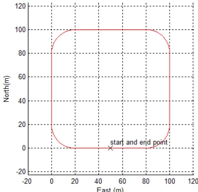
4. SIMULATION TESTS AND RESULTS A series of simulations were conducted in order to illustrate the performance of the proposed Kalman filter vs. the standard Kalman filter (KF) and the Kalman filter with the shaping filter (KF-ST) as in (Bryson and Henrikson, 1968). A 2D scenario shown in figure 1 was used to demonstrate the performance of the proposed Kalman filter algorithm with the imaging and IMU measurements. The vehicle position, velocity and heading states in the navigation frame are
T
Figure 1 shows an overview of the vehicle’s trajectory. Figure 2 and figure 3 show the vehicle’s velocity and heading profiles, respectively.
Figure 1. The top view of the vehicle trajectory
Figure 2. The velocity profile
Figure 3. The heading profile
In this example two accelerometers and one gyroscope were deviations and number of the used features.
Figure 4 2D VO measurement noise and number of features
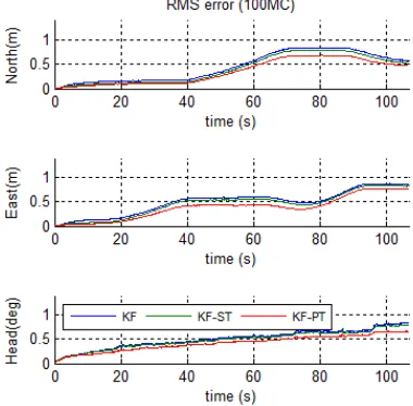
Monte Carlo (MC) simulations were used to compare the performance of the three implemented Kalman filters. Each algorithm was run 100 times. The true position and heading errors were computed for each run. Then the root-mean-square (RMS) errors across the 100 runs were computed at every epoch. The resulting error bounds were then compared with the estimated standard deviations. The figures 5 shows the true pose RMS errors computed in (a) KF (b) KF-ST and (c) the proposed KF-PT. Clearly the true KF-PT errors are smaller than the ones from KF and KF-ST.
Figure 5. True Position and Heading RMS error
Tables 1 and 2 show the average and maximum absolute errors respectively. The absolute errors in the estimates computed by KF-PT were on the average smaller compared to both KF and KF-ST.
Average KF KF-ST KF-PT
North(m) 0.451 0.404 0.349
East(m) 0.494 0.455 0.381
Heading(deg) 0.512 0.490 0.422 Table 1. Average Absolute Position and Heading Errors
Maximum KF KF-ST KF-PT
North(m) 0.851 0.793 0.690
East(m) 0.880 0.845 0.782
Heading(deg) 0.845 0.805 0.667 Table 2. Maximum Absolute Position and Heading Errors
Average Maximum
KF-PT w.r.t
KF
KF-PT w.r.t KF-ST
KF-PT w.r.t
KF
KF-PT w.r.t KF-ST
North(%) 22.6 13.8 19.0 13.0
East(%) 22.9 16.1 11.0 7.4
Heading(%) 17.7 13.9 21.1 17.1
Table 3. Position and Heading Improvement Compared to KF and KF-ST
Table 3 shows the percentage improvement in the average and maximum error estimates of PT with respect to KF and KF-ST. Clearly the estimates were improved with KF-PT in all components. The figure 6 shows the corresponding standard deviation (1) estimated from the three filters. Again KF-PT standard deviations are smaller than the ones from KF and KF-ST.
Figure 6. Estimated Position and Heading Standard Deviation Figure 7 shows the ratio of the RMS errors to estimated standard deviation. The ratios of KF-PT positions are close to 1 while KF and KF-ST ratios are less than 1. This implies that KF-PT errors closely match the estimated standard deviation while the KF and KF-ST output pessimistic estimates. Therefore the KF-PT models the pairwise-time correlated measurement correctly.
Figure 7. Ratio of RMS errors to estimated standard deviation
5. CONCLUSIONS
This paper presented a novel Kalman filtering model that can deal with pairwise time-correlated measurements. The method utilized a shaping filter that consists of Cholesky factors based on the measurement variance-covariance matrices. The augmentation was used to estimate the state vector and its associated variance-covariance matrix. The simulation results showed that the proposed Kalman filter with the time-correlated measurement noise performs better than the standard Kalman filter and the Kalman filter with the shaping filter by (Bryson and Henrikson, 1968). In the example presented the average solution of proposed Kalman filter improved by 13.8%, 16.1% and 13.9% in the North, East and heading respectively when compared to (Bryson and Henrikson, 1968). Furthermore, the Monte Carlo simulation results show that the estimated standard deviation of the solution closely matches the actual errors.
REFERENCES
Aggarwal, P; Z. Syed; A. Noureldin and N. El-Sheimy, 2010. MEMS-Based Integrated Navigation, GNSS Technology and Application series
Bierman, G. J., 1977. Factorization Methods for Discrete Sequential Estimation, ISBN 0-486-44981-5
.
Bryson, Jr., A. E. and Henrikson, L. J., 1968. Estimation using sampled data containing sequentially correlated noise. Journal of Spacecraft and Rockets, 5 (1968), 662—665.
Gelb, A., 1974. Applied Optimal Estimation, the MIT press, pp110.
Gilad A., 1985. Determining Three-Dimensional Motion and Structure from Optical Flow Generated by Several Moving Objects, IEEE Transactions on Pattern Analysis and Machine Intelligence, vol. Pami-7, No. 4, July 1985.
Grewal M. S., Angus P. Andrews, 2001. Kalman filtering: Theory and Practice Using MATLAB, Second Edition
Kun Q., N. Gopaul, J.G. Wang and B. Hu, 2012. Low Cost Multisensor Kinematic Positioning and Navigation System with Linux/RTAI, Journal of Sensor and Actuator Networks, vol. 1, issue 3, pp. 166-182.
Miller, M. M, A. Soloviev, M. U. de Haag, M. Veth, J. Raquet, T. J. Klausutis and J. E. Touma, 2011. Navigation in GPS Denied Environments: Feature-Aided Inertial Systems, NATO Research and Technology Organisation, 2011.
Mourikis A.I., S.I. Roumeliotis, J.W. Burdick, 2007. SC-KF Mobile Robot Localization: A Stochastic Cloning-Kalman Filter for Processing Relative-State Measurements, IEEE Transactions on Robotics, 23(4), pp. 717-730, August 2007. Nistér, O. Naroditsky, J. Bergen, 2006. Visual Odometry for Ground Vehicle Applications, Sarnoff Corporation, CN5300, Princeton NJ 08530 USA
Scaramuzza. D and Fraundorfer F., 2011. Visual Odometry Part I: The First 30 Years and Fundamentals, IEEE Robotics & Automation Magazine, December 2011, 18(4):80–92, 2011. Shen, Y. and J. Liu, 2005. Vision based SLAM for Robot Navigation with Single Camera, Department of Information Science and Electronic Engineering, Zheijiang University, Hangzhou 310027, China.
Williams, B. and I. Reid, 2010. On Combining Visual SLAM and Visual Odometry, Proc IEEE Int Conf on Robotics and Automation, May 2010.