A family of Pade-type approximants for accelerating
the convergence of sequences
R. Thukral
Pade Research Centre, 39 Deanswood Hill, Leeds, West Yorkshire LS17 5JS, UK Received 1 September 1997; received in revised form 7 September 1998
Abstract
We describe a collection of Pade-type methods for accelerating the convergence of sequence of functions. The con-struction and connections of Pade’s methods with other similar methods are given. We examine the eectiveness of these new methods, namely integral Pade approximant, modied Pade approximant and squared Pade approximant together with the well-established methods, namely functional Pade approximant and classical Pade approximant, for approximating the characteristic value and corresponding characteristic function. Estimates of characteristic value and characteristic function derived using integral Pade approximants are found to be substantially more accurate than other similar methods. c1999 Elsevier Science B.V. All rights reserved.
Keywords:Integral Pade approximant; Classical Pade approximant; Functional Pade approximant; Modied Pade approximant; Squared Pade approximant; Integral equation; Neumann series; Convergence acceleration
1. Introduction
In this paper, three new methods for accelerating the convergence of sequence of functions are introduced and their eectiveness is examined by determining the characteristic value and the charac-teristic function of an integral equation. These new methods use functional Pade-type approximants, where we employ the terminology “Pade-type” as introduced by C. Brezinski, which means that the denominator polynomial of the rational approximant is arbitrarily prescribed (on the contrary, in the classical Pade approach the denominator is left free in order to achieve the maximal order of interpolation). We have introduced the appropriate names for the Pade-type approximants as mod-ied Pade approximant, squared Pade approximant and integral Pade approximant. The modmod-ied Pade approximant method was the rst modication of the classical Pade approximant and this was further improved by the squared Pade approximant method. Finally, the integral Pade approximant was developed and this is shown to be a good alternative to functional Pade approximant.
The main reason for developing the appropriate denominators of the new methods was to overcome the essential diculty encountered by classical Pade approximants and functional Pade approximants.
The major drawback of these methods is the use of the minimal sensitivity principle [1, 2] and the presence of superuous zeros in the denominator. Hence, we investigated on the basis that these new methods should have a similar order and cofactors arrangement in the determinant of the denominator polynomial as classical Pade approximant and the accuracy of the functional Pade approximant. Also we use a similar principle of integrating each of the cofactors in the determinant of the denominator polynomial, which was introduced by Graves-Morris [5, 7, 11] and applied in functional Pade approximant method.
We describe the fundamentals of the denominator for each of the new Pade-type methods and the numerator is determined naturally. In order to construct these new methods we use a similar procedure as classical Pade approximant. The construction of the denominator of the modied Pade approximant method is simply obtained by integrating each of the cofactor in the determinant of the denominator polynomial of the classical Pade approximant method. This improved method overcomes the use of the minimal sensitivity principle but it lacks the desired precision and therefore we have investigated this method further. We construct the denominator of the squared Pade approximant method by squaring each of the cofactor in the determinant of the denominator polynomial of the classical Pade approximant method and then we integrate these new cofactors. The precision was good for some cases but we found that this method is not versatile. Hence, we decided to construct the denominator of the integral Pade approximant method in a dierent way to those discussed above and in previously published papers [6–8, 11]. The construction of the denominator of the integral Pade approximant method is obtained by combining the coecients of the generating function as cofactors in the determinant of the denominator polynomial. We found that the integral Pade approximant method is consistent and overcomes all the diculties encountered in the previous studies [6, 7, 11].
We begin with the generating function f(x; ) of a series of functions given by
f(x; ) = ∞
X
i=0
Ci(x)i; (1)
in which Ci(x)∈L2[a; b] are given and [a; b] is the domain of denition of Ci(x) in some natural
sense. We also suppose that f(x; ) is holomorphic as a function of at the origin = 0. Then (1) converges for values of || which are small enough. In this paper, we see how the methods of Pade-type approximation can be used to accelerate the convergence of a series having the form (1).
1.1. The integral Pade approximants method (IPA)
We dene a rational function r(x; ) to be an integral Pade approximant of type (n; k) for f(x; ) if
r(x; ) =N(x; )=D(); (2)
where N(x; ); D() are polynomials in ; N(x; )∈L2[a; b] as a function of x and
@{N}6n; @{D}6k; (3a)
D(0) = 1; (3b)
If N(x; ); D() satisfy axiom (3), then there exists a unique r(x; ) dened by (1). The proofs of existence and uniqueness are similar to that for the classical Pade approximant [4, 5, 14] and the rate of convergence is similar to functional Pade approximant. This is evident from this investigation and in all the other test examples.
For the purpose of this paper, we dene the denominator polynomial of an integral Pade approx-imant of type (n; k) as
The purpose of integrating the elements in (4) is to make the estimates of the characteristic values independent of the variable x. This is similar to the approach for the functional Pade approximant in which we overcome the serious problem, use of [1, 2], with the classical Pade approximant [7, 11]. We take the appropriate roots of denominator polynomial, given by (4), as our estimates of the characteristic value for the integral Pade approximant.
Naturally, the numerator polynomial N(x; ) follows from (3c) as N(x; ) = [D()f(x; )]n
0; (5)
where this notation, now and in the sequel, indicates that truncation at degree n in has been eected. If, in the representation (4),D(0)6= 0, thenr(x; ) dened by (2), (4) and (5) is an integral Pade approximant of type (n; k) for f(x; ).
Integral Pade approximants constructed using (3) can be laid out in a table: (0;0) (0;1) (0;2) · · ·
and this concept is similar to the classical Pade approximants [5].
Conjecture 1.1 (Integral Pade approximant). Let
f(x; ) =N(x; )=D() (7)
be a meromorphic function with precisely k nite poles. Then; for all n suciently large; there exists a unique rational function r(x; ) of type (n; k) which interpolates to f(x; ). Hence
lim
n→∞
Nn(x; )
Dn()
Summaries of the advantages of integral Pade approximants are as follows:
(i) We do not have to assign a particular value of x in the Neumann series, to obtain an estimate of the characteristic value using classical Pade approximant [7, 11].
(ii) Integral Pade approximants produces a substantially more accurate estimates than the classi-cal Pade approximant, the modied Pade approximant and the other two methods considered previously, namely Fredholm determinant and Rayleigh–Ritz [7, 11].
(iii) The order of the denominator polynomial of an integral Pade approximant is half the order of the denominator polynomial of the functional Pade approximant. Therefore, an integral Pade ap-proximant does not possess superuous zeros, which was a serious problem with the functional Pade approximant as noted by the investigators [6, 7, 11].
(iv) We do not have to construct a further method, known as the hybrid functional Pade approximant, to obtain the characteristic function [6, 7, 11].
(v) From the last two advantages it is established that the method of the functional Pade approxi-mants needs much more numerical computation than integral Pade approxiapproxi-mants.
(vi) Integral Pade approximant is applicable to a wider class of generating functions. We found a major drawback of the squared Pade approximant is that the numerical performance of this method is not suitable when the generating function possesses an alternating or a negative power series.
(vii) Integral Pade approximant is simpler and more eective method for obtaining the characteristic values and the characteristic functions than other similar methods.
1.2. The modied Pade approximant method (MPA)
A modied Pade approximant of type (n; k) for the given power series (1) is the rational function
r(x; ) =A(x; )=B(); (9)
where A(x; ); B() are polynomials in ; A(x; )∈L2[a; b] as a function of x and
@{A}6n @{B}6k; (10a)
B(0) = 1; (10b)
A(x; )−B()f(x; ) = 0(n+1): (10c)
Naturally, the numerator polynomial A(x; ) follows from (10c) as
A(x; ) = [B()f(x; )]n0: (12)
Each approximant of the sequence of (n; k) type modied Pade approximant has preciselyk poles. We take the zeros of (11) as our estimates of the characteristic value for the modied Pade approximant.
1.3. The squared Pade approximant method (SPA)
A squared Pade approximant of type (n; k) for the given power series (l) is the rational function
r(x; ) =G(x; )=H(); (13)
where G(x; ), H() are polynomials in , G(x; )∈L2[a; b] as a function of x and
@{G}6n; @{H}6k; (14a)
H(0) = 1; (14b)
G(x; )−H()f(x; ) = 0(n+1): (14c)
The construction of the denominator polynomial of the squared Pade approximant of type (n; k) is given as
Naturally, the numerator polynomial G(x; ) follows from (14c) as
G(x; ) = [H()f(x; )]n0: (16)
Each approximant of the sequence of (n; k) type Pade approximant has preciselyk poles. We actually take the square root of the zeros formed by (15) as our estimates of the characteristic value.
approximations leading to an innite power series solution. In the process we make two distinct com-parisons of the estimates derived using the integral Pade approximant. First, we compare estimates formed using the row sequence of an integral Pade approximant of type (n;1) with corresponding estimates derived from the modied Pade approximant of type (n;1), the squared Pade approximant of type (n;1), the functional Pade approximant of type (n;2) and the classical Pade approximant of type (n;1). Then we compare estimates based on another row sequence of an integral Pade ap-proximant of type (n;2) with corresponding estimates derived from the modied Pade approximant of type (n;2) the squared Pade approximant of type (n;2), the functional Pade approximant of type (n;4) and the classical Pade approximant of type (n;2). In Section 6 we illustrate the precision of a particular characteristic function of integral Pade approximant. The eectiveness of these new methods for accelerating the convergence of a sequence of functions was investigated in the context of the Neumann series of an integral equation. The method of integral Pade approximants proved to be the most eective of the methods considered.
2. The classical Pade approximant method (CPA)
A classical Pade approximant of type (n; k) for the given power series (l) is the rational function
r(x; ) =U(x; )=V(x; ); (17)
where U(x; ); V(x; ) are polynomials in ; U(x; )∈L2[a; b] as a function of x and
@{U}6n; @{V}6k; (18a)
V(0) = 1; (18b)
U(x; )−V(x; )f(x; ) = 0(n+k+1): (18c)
The construction of the denominator polynomial of classical Pade approximant of type (n; k) is given as
V(x; ) =
Cn−k+1(x) Cn−k+2(x) · · · Cn+1(x) Cn−k+2(x) Cn−k+3(x) · · · Cn+2(x)
..
. ... ...
k k−1
· · · 1
; (19)
provided V(x;0)6= 0 and Ci(x) are coecients of (1).
Naturally, the numerator polynomial U(x; ) follows from (18c) as
U(x; ) = [V()f(x; )]n
0: (20)
Each approximant of the sequence of (n; k)-type Pade approximant has precisely k poles. To deter-mine these zeros, in order to estimate the characteristic value, we must assign a particular value of x in the Neumann series and this is usually done using the principle of minimal sensitivity [1, 2].
3. The functional Pade approximants method (FPA)
We dene a rational function r(x; ) to be a functional Pade approximant of type (n;2k) for f(x; ) if
The asterisk in (22c) denotes the functional complex conjugate.
If p(x; ),q(), satisfy (22a)–(e), thenr(x; ) dened by (1) is unique; the questions of existence, uniqueness and degeneracy are treated in [9]. The explicit formula for the denominator polynomial is given by
The elements of (23) are dened by
Mij=
We know that the polynomials produced by (23) are strictly positive for ∈R and their zeros occur in complex conjugate pairs close to the real axis [6, 7, 11]. Ideally, we take the real parts of the zeros of q() as our estimates of the characteristic values c.
The numerator polynomial p(x; ) follows from (22e) as
p(x; ) = [q()f(x; )]n
0: (25)
In addition, the denominator polynomial of a hybrid functional Pade approximant is dened in terms of the roots of the denominator of the corresponding functional Pade approximant [6, 7, 11]. We actually take the real parts of the roots of the functional Pade approximant and express the hybrid functional Pade approximant of type (n; k) as
qH() =
k
Y
i=1
(−R
i ): (26)
The associated numerator polynomial is dened as
pH(x; ) = [f(x; )qH()]n0: (27)
Since n and k govern the degree of the numerator and denominator, respectively, we express the hybrid functional Pade approximant of type (n; k) as
rH(x; ) =pH(x; )=qH(): (28)
We nd that (28) is identical to the integral Pade approximant (2) for k= 1. It is obvious that the hybrid functional Pade approximant is dependent on functional Pade approximant and therefore requires much more numerical computation than the integral Pade approximant. We can easily prove this by comparing the dimensions of the determinant and the degree of the denominator polynomial of functional Pade approximant and integral Pade approximant, which are given by (23) and (4), respectively.
4. Equivalence of the estimates
Here we shall observe how three methods, namely integral Pade approximant, the squared Pade ap-proximant and the functional Pade apap-proximant produce similar estimates of the characteristic value. We shall do this by showing that the limit of the poles of the respective denominator polynomial satises identical equations.
First we begin by expanding (4), the denominator polynomial of the integral Pade approximant of type (n;1):
D() =
Z b
a
Cn(x)Cn−1(x) dx
Z b
a
Cn2(x) dx
1
;
which gives
D() =
Z b
a
Cn(x)Cn−1(x) dx−
Z b
a
C2
n(x) dx: (29)
The characteristic value of the integral Pade approximant of type (n;1) is calculated by solving (29) and thus we have
=
Z b
a
Cn(x)Cn−1(x) dx
, Z b
a
Similarly, expanding the denominator polynomial of the functional Pade approximant of type (n;2),
Solving (31) by a standard quadratic formula and simplifying gives rise to
=[
We know from previous studies [6, 7, 11] that (32) produces a pair of complex conjugates which are close to the real axis, that is
"
Therefore, the estimate of the characteristic value of the functional Pade approximant of type (n;2) method is given by
=
Alternatively, we can nd the estimates of the functional Pade approximant by dierentiating (31) w.r.t. and with a convenient normalisation we obtain (35) [8, 11].
which gives
The characteristic value of squared Pade approximant of type (n;1) is based on solving (36); thus we have
If we rearrange (34), we have
lim
and substituting the right-hand side of (38) into (37) we obtain
=
It has been established in [5, 6, 8, 10] that the zeros, that is characteristic value, of the functional Pade approximant converges as
lim
n→∞
n=2: (40)
This result also applies to the squared Pade approximant.
However, we actually take the square root of (37) as our estimates of the characteristic value
=
Therefore, we expect that, for all n suciently large, (41) is equivalent to (30). It should be noted that this is true mathematically, but we nd a serious problem numerically that is when the generating function possesses an alternating or a negative power series.
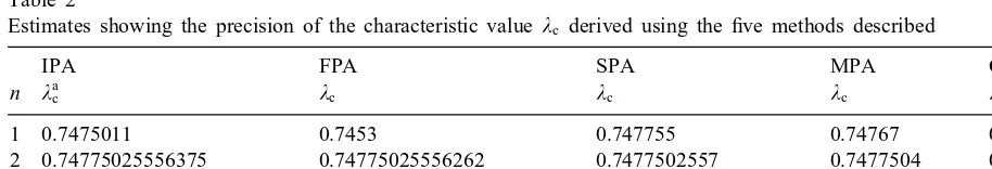
Mathematically, we have demonstrated the fact that these three methods produce a similar accuracy for the estimates of the characteristic value, that is (30), (35) and (41) are similar for the rst row sequence. We conjecture that these three methods produce identical estimates for any type of row sequence. However, numerically we nd that the integral Pade approximant has better precision than the squared Pade approximant and the functional Pade approximant. This is empirically evident from Table 2.
5. Application to an integral equation
generalised by illustrating the eectiveness of these new methods for determining the characteristic values and the characteristic function of a familiar linear integral equation in the following example. We investigate the convergence of sequences of these new methods for the Neumann series solution of the linear integral equation
f(x; ) = 1 +
Z 1
0
k(x; y)f(y; ) dy; (42)
where
k(x; y) =
1 +x−y; 06y6x61; 1 +y−x; 06x6y61:
This integral equation is a Fredholm of the second kind with a nondegenerate kernel and has been previously considered by Graves–Morris [7] and Coope and Graves–Morris [6].
The characteristic functions of this equation can be found by converting it to a second-order ordinary dierential equation [3]. The explicit solution of (42) is
f(x; ) = 2 cosh(x−1=2)
2 cosh=2−3sinh=2; (43)
where =√2. The denominator of (43) is analytic as a function of and has just one simple zero at c= 1:22290658: : :, corresponding to a single characteristic value c= 0:7477502556: : :.
It is familiar that the Neumann series of (42) converges for ||¡c [12]. The rst few terms of
this series are
f(x; ) = ∞
X
i=0
Ci(x)i= 1 +
"
5 4 +
x−1 2
2#
+
"
161 96 +
5 4
x−1 2
2
+1 6
x−1 2
4#
2+· · ·;
(44)
as may be found by iteration of (42).
We make two distinct comparisons of the estimates derived using the integral Pade approximants. First, we compare estimates formed using the row sequence of the integral Pade approximant of type (n;1) with corresponding estimates derived from the classical Pade approximant of type (n;1), the modied Pade approximant of type (n;1), the squared Pade approximant of type (n;1) and the functional Pade approximant of type (n;2). The results in Table 1 are the estimates of the characteristic value for each of the ve iterative methods described and we nd that the estimates from the integral Pade approximant gives better approximations that the classical Pade approximant, the modied Pade approximant and it is similar to the functional Pade approximant and the squared Pade approximant. The results in Table 2 are the estimates of the characteristic value, but showing results derived from another row sequence of the integral Pade approximant of type (n;2) and with corresponding estimates derived from the classical Pade approximant of type (n;2), the modied Pade approximant of type (n;2), the squared Pade approximant of type (n;2) and the functional Pade approximant of type (n;4). We see that the row sequence of the integral Pade approximants gives better approximation than the other methods, including the functional Pade approximants. In each case, the comparisons with other methods were made using a similar amount of data, which is, using a similar number of terms of (44).
Table 1
Estimates showing the precision of the characteristic valuec derived using the ve methods described
IPA = FPA SPA MPA CPA
n ac c c c
1 0.74766 0.7488 0.75 0.8
2 0.74775011 0.747752 0.74766 0.745
3 0.7477502553 0.7477502583 0.747754 0.74785
4 0.7477502555635 0.747750255568 0.74775011 0.747746
5 0.7477502555638444 0.747750255563853 0.747750261 0.74775043
a
The exact value of c= 0:747750255563845043: : : .
Table 2
Estimates showing the precision of the characteristic valuec derived using the ve methods described
IPA FPA SPA MPA CPA
n ac c c c c
1 0.7475011 0.7453 0.747755 0.74767 0.7486
2 0.74775025556375 0.74775025556262 0.7477502557 0.7477504 0.74774 3 0.747750255563845035 0.74775025556384496 0.747750255563858 0.7477502545 0.7477504 4 0.7477502555638450433881 0.7477502555638450433815 0.747750255563845045 0.74775025557 0.74775025
a
The exact value of c= 0:74775025556384504338894: : : .
theorem [13]. Likewise, the proof that the functional Pade approximant estimates shown in the Table 1 converge geometrically to the characteristic value, follows as a consequence of the row conver-gence theorem of Graves–Morris and Sa [10]. All these mathematical results are empirically evident from Tables 1 and 2. It is also clear that the integral Pade approximant method converges much faster than the other methods. This is due to the standard theory of Fredholm integral equations of the second kind [12, 15], that is expressed by
f(x; ) =g(x) +
Z b
a
k(x; y)f(y; ) dy; (45)
it is known that when g(x)∈L2[a; b] and k(x; y) is an L
2 kernel,
f(x; y) =P(x; )
Q() ; (46)
where
(i) P(x; ) is holomorphic as a function of , (ii) P(x; )∈L2[a; b] for a xed ,
(iii) Q() is holomorphic function of , (iv) Q(0)6= 0.
of estimates of the characteristic values derived from the integral Pade approximants as shown in Tables 1 and 2.
6. Precision of the approximate solution
In Fig. 1 we display the exact (analytic) solution and its approximations obtained using the in-tegral Pade approximant of type (2;1), the modied Pade approximant of type (2;1), the squared Pade approximant of type (2;1) and the functional Pade approximant of type (2;2). Also in Fig. 1 we see a remarkable precision of the integral Pade approximant, where graphically there is no signicant dierence between the exact and the integral Pade approximant. Accordingly, in Table 3, we show the errors incurred by the integral Pade approximant, the modied Pade approxi-mant, the squared Pade approximant and the functional Pade approximant methods for x= 0(0:1)0:5 in the solution of (42). We list the appropriate rational functions displayed.
Solution of the integral equation (42) using the integral Pade approximant of type (2;1) is
r(x; ) =N(x; )
D() =
1 + x2
−x+ 4399 27045
+ 1 6x
4
−1 3x
3+ 4399 27045x
2+ 217
54090x− 217 36060
2
1−7233754090 : (47)
Fig. 1. The analytic solution (exact) of (42) for = 1. The curves IPA and MPA are indistinguishable from the exact curve. Whereas the curve FPA is perceptibly dierent and SPA is beyond the exact curve.
Table 3
Errors occurring in the solution of (42) using the integral Pade approximant, the modied Pade approximant, the squared Pade approximant and the functional Pade approximant method
IPA MPA SPA FPA
x = 1 = 1 = 1 = 1
0 −0.00088 −0.0036 −3.39 0.069
0.1 −0.00066 −0.0032 −3.19 0.050
0.2 −0.00021 −0.0026 −3.04 0.013
0.3 0.00031 −0.0020 −2.93 −0.026
0.4 0.00070 −0.0016 −2.86 −0.053
Solution of (42) based on the squared Pade approximant of type (2;1) is
Solution of (42) based on the functional Pade approximant of type (2;2) is
r(x; ) =p(x; )
Solution of (42) based on the modied Pade approximant of type (2;1) is
r(x; ) =A(x; )
The rational functions above were suitably normalised.
It has been established in previous studies [6, 7, 11] that the estimates of characteristic function based on the functional Pade approximants are inferior to those from the hybrid functional Pade approximants. The reason for the poor performance of the functional Pade approximants for the estimation of the characteristic function is that the denominator polynomials (11) possess superuous zeros, and thus the hybrid functional Pade approximant method was introduced. We do not use the hybrid functional Pade approximant, not because it produces identical results to the integral Pade approximant, but because of much more numerical computation involved in deriving it. Furthermore, we have found that the precision of the characteristic function for the squared Pade approximant method is considerably smaller than the integral Pade approximant. Finally, although the approximate solution for the characteristic function for the modied Pade approximant is satisfactory, it lacks the precision of the integral Pade approximant.
7. Remarks and conclusion
Three new methods for producing a sequence of rational approximations to the solution of a linear integral equation have been described and their eectiveness has been investigated in many examples. These new methods are essentially for accelerating the convergence of a sequence of functions. In the context of a familiar linear integral equation, the method of integral Pade approximants is shown to be much more ecient in calculating the characteristic value and substantially more accurate for calculating the approximate solution than other similar techniques.
Acknowledgements
I am greatly indebted to an anonymous referee and Professor D.B. Ingham for helpful comments on this paper.
Appendix. Application to another integral equation
We illustrate the eectiveness of new methods by taking another well known example. We inves-tigate the convergence of sequences of integral Pade approximants for the Neumann series solution of the linear integral equation
f(x; ) = 1 +
Z 1
−1
k(x; y)f(y) dy; (A.1)
where
k(x; y) =
(
8−1
(1 +y)(1−x); −16y6x61; 8−1
(1 +x)(1−y); −16x6y61:
This integral equation is a Fredholm of the secod kind with a nondegenerate kernel previously considered by Graves-Morris and Thukral [11].
The characteristic functions of this equation can be found by converting it to a second-order ordinary dierential equation [3]. The explicit solution of (1) is
f(x; s) = sin[2
−1
s(1 +x)]; s∈ ℵ;
Table 4
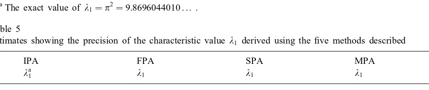
Estimates showing the precision of the characteristic value1 derived using the ve methods described
IPA= FPA SPA MPA CPA
n a1 1 1 1
1 10 10.95 12 8
2 9.871 9.877 10 9.6
3 9.86962 9.86969 9.88 9.84
4 9.8696046 9.8696054 9.871 9.866
aThe exact value of
1=2= 9:8696044010: : : .
Table 5
Estimates showing the precision of the characteristic value1 derived using the ve methods described
IPA FPA SPA MPA CPA
n a
1 1 1 1 1
1 9.871 9.24 10.03 10.25 10.14
2 9.8696046 9.869609 9.86964 9.8751 9.878
3 9.8696044013 9.8696044025 9.86960444 9.86975 9.8699
4 9.8696044010896 9.869604401091 9.86960440115 9.869609 9.86962 5 9.8696044010893593 9.869604401089361 9.86960440108946 9.8696046 9.8696051
aThe exact value of
Table 6
Estimates showing the precision of the characteristic value3 derived using the three methods described
IPA FPA SPA MPA CPA
n a3 3 3 3 3
1 — — — — —
2 90.1 104.5 126.1 170.1 64.79
3 88.97 90.26 90.99 102.1 78.31
4 88.845 88.999 89.07 92.6 84.52
5 88.8289 88.848 88.858 90.1 87.15
aThe exact value of
3= 92= 88:8264396: : : .
with corresponding characteristic value
s= (s)2; s∈ ℵ:
References
[1] C. Alabiso, P. Butera, G.M. Prosperi, Resolvent operator, Pade approximation and bound states in potential scattering, Nuovo Cim. 3 (1970) 831–839.
[2] C. Alabiso, P. Butera, G.M. Prosperi, Variational principles and Pade approximants. Bound states in potential theory, Nucl. Phys. B 31 (1971) 141–162.
[3] C.T.H. Baker, The Numerical Treatment of Integral Equations, Oxford University Press, Oxford, 1978. [4] G.A. Baker, Essentials of Pade approximants, Academic Press, New York, 1975.
[5] G.A. Baker, P.R. Graves-Morris, Pade approximants, Cambridge University Press, Cambridge, UK, 1996.
[6] I.D. Coope, P.R. Graves-Morris, The rise and fall of the vector epsilon algorithm, Numer. Algorithm 5 (1993) 275–286.
[7] P.R. Graves-Morris, Solution of integral equations using generalised inverse, function-valued Pade approximants I. J. Comp. Appl. Math. 32 (1990) 117–124.
[8] P.R. Graves-Morris, A review of Pade methods for the acceleration of convergence of a sequence of vectors. Appl. Numer. Math. 15 (1994) 153–174.
[9] P.R. Graves-Morris, C.D. Jenkins, Degeneracies of generalised inverse, vector-valued Pade approximants, Constr. Approx. 5 (1989) 463– 485.
[10] P.R. Graves-Morris, E.B. Sa, Row convergence theorems for generalised inverse, vector-valued Pade approximants, J. Comput. Appl. 23 (1988) 63–85.
[11] P.R. Graves-Morris, R. Thukral, Solution of integral equations using function-valued Pade approximants II, Numer. Algorithms 3 (1992) 223–234.
[12] B.L. Moiseiwitsch, Integral Equations, Longman, New York, 1977.
[13] R. de Montessus de Ballore, Sur les fractions continues algebriques, Bull. Soc. Math. France 30 (1902) 28–36. [14] E.B. Sa, An extension of R. de Montessus de Ballore’s theorem on the convergence of interpolating rational
functions, J. Approx. Theory 6 (1972) 63– 67.