Ecological Economics 36 (2001) 513 – 531
ANALYSIS
Interrelationships between income, health and the
environment: extending the Environmental Kuznets Curve
hypothesis
Lata Gangadharan
a,*, Ma. Rebecca Valenzuela
baDepartment of Economics,Uni6ersity of Melbourne,Melbourne,Vic.3010,Australia bDepartment of Economics,Monash Uni6ersity,Vic.3145,Australia
Received 4 April 2000; received in revised form 19 September 2000; accepted 20 September 2000
Abstract
This paper examines the link between the health indicators and the environmental variables for a cross-section of countries widely dispersed on the economic development spectrum. While environment and income are seen to have an inverted-U shaped relationship (Environmental Kuznets Curve (EKC) hypothesis), it is also well established that environment and health are positively related. Our study focuses on the implications of this for the relationship between health and income. In the early phases of income growth, the gains in health and the losses in environmental quality could cancel each other out and this challenges the idea that as incomes increase health would always improve. To empirically analyse these issues, we estimate a two-stage least squares model that focuses on the impact of income and the environment on health status, with environment being an endogenous variable. Our results show that the environmental stress variable has a significant negative effect on health status. At the same time, gross national product (GNP) levels are shown to vary positively with health status variables. We find that the health gains obtained through improved incomes can be negated to a significant extent if the indirect effect of income acting via the environment is ignored. Research findings in this regard would be a useful policy instrument towards maximising both the environmental and health gains that come with economic growth and development. © 2001 Elsevier Science B.V. All rights reserved.
Keywords:Environmental stress; Health indicators; Income levels
JEL classification:O11; Q25; C30
www.elsevier.com/locate/ecolecon
* Corresponding author.
E-mail addresses: [email protected] (L. Gangadharan), [email protected] (M.R. Valenzuela).
L.Gangadharan,M.R.Valenzuela/Ecological Economics36 (2001) 513 – 531
514
1. Introduction
Is economic growth part of the solution rather than the cause of environmental problems? This question has been raised very often in recent years as empirical evidence in support of the Environ-mental Kuznets Curve (EKC) hypothesis mount.1 The EKC (Grossman, 1995; Grossman and Kreuger, 1995) describes the relationship between declining environmental quality and income as an inverted-U, that is, in the course of economic growth and development, environmental quality initially worsens but ultimately improves with im-provements in income levels. For instance, Torras and Boyce (1998) show that the level of air pollu-tants (sulphur dioxide and smoke) peak at a per capita income in the neighbourhood of US $4000, after which they start falling.
One of the explanations for the EKC relation-ship is that the environment can be thought of as a luxury good. In the early stages of economic development, a country would be unwilling to trade consumption for investment in environmen-tal regulation, hence environmenenvironmen-tal quality de-clines. Once the country reaches a threshold level of income, its citizens start to demand improve-ments in environmental quality and this leads to the implementation of policies for environmental protection and, eventually, to reductions in pollu-tion. Increasing levels of pollution are thus strongly associated with both poor and develop-ing economies, while declindevelop-ing levels of pollution are more commonly observed for their developed counterparts.2
Another explanation of the EKC hypothesis is that countries pass through techno-logical life cycles, as they move from agriculture-based economies to service-agriculture-based systems. As the service sector is associated with lower environ-mental impact, this transition from high polluting to low polluting technology leads to less
environ-mental stress. Hence, in the long run, pollution levels are expected to improve with incomes. This argument has been used to justify the pursuit of growth strategies that do not give due consider-ation to their effect on the environment.
In this paper, we argue that this strategy is not justified and provide some evidence to support our case. We test the hypothesis that larger eco-nomic and social gains can be attained by an economy if the growth strategy adopted incorpo-rates, rather than ignores, environmental con-cerns. To do this, we include health as the intervening variable in the analysis. While envi-ronment and income are seen to have an inverted-U shaped relationship, it is also well established that health and environment are positively re-lated. What does this imply for the relationship between health and income? It is possible that in the early phases of income growth, the gains in health and the losses in environmental quality cancel each other out and this challenges the idea that as incomes increase, health would always improve.
In view of the above, we argue in this paper that the recorded health gains brought about by the improvement in income levels do not repre-sent the total realisable health benefits from hav-ing higher per capita income. Without the appropriate environmental protection policies, damages to a country’s physical environment are incurred during the process of income growth and economic development. This negatively affects the health and well-being of individuals in the country and the aggregated impact could negate some of the health gains already derived, and hence dampen achievement levels in the health area. If we find that this argument has some empirical support, it would imply that development policies addressing environmental issues are effectively also addressing the health issues of the economy. In that case, policies that pursue economic devel-opment cannot afford to ignore environmental issues, particularly in the early phases of eco-nomic growth.
We look at recent evidence from a cross-section of countries to determine if this is indeed the case. While there are some studies (for example, Crop-per et al., 1997) that look at the incidences of air
1The original Kuznets curve refers to an inverted-U shaped
relationship between per capita income and inequality ob-served by Kuznets (1955).
2For example, Grossman and Kreuger (1995) found
L.Gangadharan,M.R.Valenzuela/Ecological Economics36 (2001) 513 – 531 515
or water pollution-related diseases in a particular region or country, this is one of the first papers to analyse the link between the health indicators and the environmental variables for a cross-section of countries widely dispersed on the economic devel-opment spectrum.
The major contributions of this paper are the following.
1. To establish the link between health and envi-ronment. While this link has been suggested before, to the best of our knowledge it has not been explored for different countries.
2. To explore the differential impact on health of several environmental stress variables. The standard practice is to focus on just one vari-able, normally CO2 emissions. We attempt to
make our findings and conclusions more ro-bust by including several other pollutants and environmental damage indicators in the analysis.
3. To analyse the shape of the EKC curve and the health relationship using alternative func-tional forms to determine which among them best fits the data.
The rest of the paper is organised as follows. Section 2 surveys the related literature on the relationship between income levels and environ-mental stress and the link between income levels and health status. Section 3 describes the analyti-cal framework and the estimation methodology used in the paper. Section 4 summarises the data used in the analysis. Section 5 discusses the results from the estimation, and Section 6 concludes.
2. Related literature survey
Panayotou (1993), Selden and Song (1994) and Grossman and Kreuger (1995) presented initial evidence that some pollutants follow an inverted-U shaped curve with respect to income. This was widely interpreted (for example, World Bank, 1992) to mean that the surest way to improve a country’s physical environment is to increase in-come levels. More recent work has focused on factors other than income as explanatory vari-ables in analysing variations in environmental stress in different countries. Kaufmann et al.
(1998), Torras and Boyce (1998), Suri and Chap-man (1998)and Agras and ChapChap-man (1999) argue that the EKC’s previously estimated could be due to important missing variables. Kaufmann et al. (1998) stress the importance of spatial intensity of economic activity, Torras and Boyce (1998) ex-plore the effects of social factors like civil rights, income inequality and education, while Suri and Chapman (1998)and Agras and Chapman (1999) find that trade-related variables and the price of energy have significant explanatory power. Most of the papers mentioned use linear or a log linear functional relationship between emissions and in-come. An exception is Galeotti and Lanza (1999), which studied relationships based on the gamma distribution. The current state of the research on the EKC is unable to conclude if the EKC hy-pothesis is confirmed or rejected.
With regards to health, there exists a large literature that has analysed the relationship be-tween income and health using cross-country data (for example, Gerdtham et al., 1992; Chakrabarti and Rao, 1999). A number of previous studies in this literature have found an economically and statistically significant and negative income elas-ticity of infant mortality rate (see for example, Flegg, 1982; Parpel and Pillai, 1986; Hill and King, 1992; Kakwani, 1993; Subbarao and Raney, 1995; Pritchett and Summers, 1996). Simi-larly, research on life expectancy and income has shown that there is a positive relationship between increases in income and life expectancy, with in-come elasticity of life expectancy estimated to be significant and positive (Preston, 1980; Hill and King, 1992). Most of these studies also control for other factors that affect health status such as the accessibility of health services and education lev-els of the population.
3. Analytical framework
L.Gangadharan,M.R.Valenzuela/Ecological Economics36 (2001) 513 – 531
516
the rise in general standard of living, including improved access to educational opportunities and health services. One’s health is also seen as depen-dent on the quality of his or her physical environ-ment — such as the amount of air pollution or the quality of drinking water. At the same time, the quality of a country’s physical environment is a result of certain growth factors in the economy. These include, for instance, the more intensive use of land, forest and water resources to increase overall economic production. Air pollution levels are also bound to increase as production levels rise. Increase in population numbers is another important factor in this context.
The relationships discussed above are sum-marised in the following general model:
Hi=f(Xi,Ei(Xi,Zi),Wi) (1)
which states that an economy’s health status (Hi)
depends on its level of economic growth (Xi), the
quality of its environment (Ei) and other social
factors (Wi) including the provision and access to
health facilities. Zi is used to denote the factors
that determine the quality of the environment. Within this framework, we test the relevance of the EKC hypothesis, captured in the termEi (Xi,
Zi), and how it impacts on the health outcomes
for a country’s population.
To empirically analyse these issues, the follow-ing econometric model is formulated for country i:
Ei=b0+b11Xi+b12Xi
2
+b13Xi 3
+b2Zi+ei (2)
Hi=a0+a1Xi+a2Wi+a3Ei+ui (3)
whereEirefers to the overall level of
environmen-tal stress in the economy; Hi refers to health
status of the population;Xi pertains to the
coun-try’s level of economic growth;Zi, are non-income
variables that impact on the environment;Wi, are
variables that directly influence health such as provision and access to medical facilities, etc.;ui,
ei, are the error terms.
Eq. (2) is the EKC, where the dependence of environmental quality on economic growth is rep-resented in a cubic relationship. The inverted-U shaped EKC requiresb11to be positive andb12to be negative. A cubic income term is added to test
the proposition from recent research that environ-mental quality tends to increase once again with extremely high incomes (De Bruyn et al., 1998). The upward bend of the Kuznets curve at the very high-income levels will be captured by the b13 term, which is expected to have a positive sign. The Zi term captures the effects of non-income
variables such as population levels, literacy rates and income inequality, which are thought to sig-nificantly influence environmental outcomes. For example, countries with higher population densi-ties are expected to suffer from greater environ-mental stress as there would be more people sharing the existing environmental resources. A country’s level of urbanisation is also thought to negatively impact on the environment, although it is possible that urbanisation can bring improved waste disposal and sanitation provisions for the urban areas, and hence mitigate the detrimental environmental effects of an increase in popula-tion. Further, there are strong grounds for believ-ing that the education levels of the population are positively associated with better environmental quality, while is not clear in which direction the gap between the rich and the poor influences the environment. In previous research, increases in the inequality of income distribution have been associated with higher levels of pollution, as those who benefit from pollution-generating activities are better able to prevail against those who bear the costs (Torras and Boyce, 1998). However, this hypothesis has been challenged by Scruggs (1998), who suggests that it is impossible to make gener-alisations about the effect of income distribution on environmental degradation without having more information about the preferences of differ-ent income groups.
Eq. (3) postulates that the population’s overall health and general well-being is dependent on three factors, the country’s level of economic growth; the availability and accessibility of medi-cal facilities; and the quality of the country’s physical environment. Xi and Ei are the same
variables defined in Eq. (2) while Wi captures all
L.Gangadharan,M.R.Valenzuela/Ecological Economics36 (2001) 513 – 531 517
The quality of the physical environment is in-cluded here as an endogenous variable. We expect that health indicators would show an improve-ment with better availability of health care ser-vices and with higher rates of child immunisation. Urbanisation being an indicator of modernisation could lead to improved health, as there might be easier access to sophisticated health facilities. However, it is also possible that the same could impact negatively on health quality as urbanisa-tion very often leads to overcrowding, poor sani-tation levels and hence more health ailments. We expect higher educational levels to improve health quality as education lowers the cost of informa-tion, and people with higher levels of education might have a better understanding of the value of public health infrastructure and are better able to locate and utilise these services. In particular, education has often been cited for its strong effect on reducing child mortality (for example, Melling-ton and Cameron, 1999).
In the above model, the structural equations are clearly identified given thatEiandHiare the only
endogenous variables in the system while the rest (Xi, Zi and Wi) are taken to be exogenous. The
equations are then estimated using general two-stage least squares estimation methods. The re-sults obtained are subjected to a robustness test with regards to functional forms and to different assumptions made regarding the type and nature of the variables used. The coefficients from the estimated equations will indicate if environmental variables play an important role in improving health outcomes in a country.
4. Data
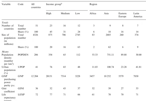
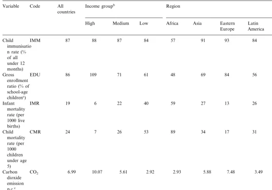
The data used in this paper are obtained from the World Development Indicators (1998), com-piled by the World Bank. Summary statistics of these data and the units of measurement used are presented in Table 1. There are a total of 51 countries included in the analysis, covering more than 70% of the world’s population (Appendix A).3
Twenty-two of the 51 countries (43%) come from the high-income OECD set, but the population composition is dominated by those in the low-in-come countries, with the inclusion of China and India in this group.
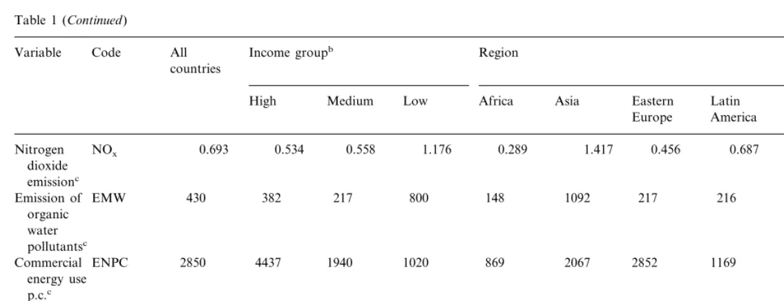
There are a number of environmental stress variables that are available for analysis. The air pollutants for which data are available are carbon dioxide (CO2), sulphur dioxide (SO2), nitrogen oxides (NOx) and total suspended particulates (TSP).4
Commercial energy use (ENPC) is taken to be another environmental indicator. For water pollution, we use data on emission levels of or-ganic pollutants (EMW) while data on deforesta-tion rates (DEFRTE) have also been obtained from the World Bank. CO2emissions and ENPC are very high for richer countries compared with low-income countries. Other air pollutants like SO2, NOx and TSP are significantly higher for low-income countries than for the high-income countries in the sample. This could be due to the fact that richer countries have already in place environmental regulations targeting these pollu-tants, while this has yet to be implemented for poorer countries. EMW and DEFRTE are much higher for low-income countries for similar reasons.
The link of the environment with the country’s level of economic growth is analysed using the country’s gross national product (GNP) per cap-ita, purchasing power parity, as the proxy vari-able for the latter.5 Population factors are controlled for the estimation through the
coun-4The data for SO
2, NOxand TSP were provided at the city
level not the country level. We obtain the country level data using the city’s population as a proportion of the country’s population.
5It is acknowledged here that gross national product is just
one aspect of economic growth and development, and that other more broad based measures (for example, the Human Development Index or HDI) are available. We nonetheless use GNP in this analysis to facilitate comparison with previous EKC studies. It is noted that GNP is highly correlated with HDI values for the countries covered in this study (r=0.82), therefore, results should be robust between these two vari-ables. For more details on the importance of alternative measures of income and growth on the EKC relationship, see Munasinghe (1999).
3The countries in the sample are listed in the Table of
L
.
Gangadharan
,
M
.
R
.
Valenzuela
/
Ecological
Economics
36
(2001)
513
–
531
518
Table 1
Variable means and summary statisticsa
Income groupb Region
Code All Variable
countries
Medium Low Africa Asia Eastern Latin Middle OECD
High
East Europe America
Totals
16 12 3 9 8
Number of Total 51 23 7 2 22
number countries
6 18 16 14
45 4
100 31 24 43
Share (%)
4326 875 706 2745 83 2685 260 374
Size of Total 122 802
number population (in millions)
2 62 6 9 3
Share (%) 100 20 16 63 19
Means
Population POPDEN 206 354 65 112 53.33 751.11 89.88 30.00 50.00 117
density (number per km2)
65 48 11.03 100.74 23.28
UPOP 41 76 41.81 31.90 74
Urban population (%)
20151 7514 3228 3457 10 252
GNP GNP 12 204 5579 7830 4110 18 733
purchasing power parity p.c.
37 52 39 27
GINI 36 32 53 38 32
Gini 43
coefficient
LEXP 77 71 66 61 70 70 71 68 76
Life 72
expectancy (years)
71 62 58 42 63 65
HLE 64
Healthy life 65 60 71
expectancy (years, 1997–1999)
202 257 157 19 26 72 309 147 126 263
DOC Physicians/
L
.
Gangadharan
,
M
.
R
.
Valenzuela
/
Ecological
Economics
36
(2001)
513
–
531
519
Table 1 (Continued)
Income groupb Region
Code All
Variable
countries
Africa Asia Eastern Latin Middle
Low OECD
Medium High
Europe America East
IMM 87 88 87 84 57 91 93 84 95 87
Child immunisatio n rate (% of all under 12 months)
86 109 71 61
Gross EDU 48 69 84 56 72 109
enrollment ratio (% of school-age childrenc)
Infant IMR 19 6 22 40 59 27 13 26 44 8
mortality rate (per 1000 live births)
9
CMR 24 7 26 53 89
Child 34 17 31 52
mortality rate (per 1000 children under age 5)
10.07 5.61
Carbon CO2 6.99 2.92 2.93 5.88 7.48 3.49 2.95 9.30
dioxide emission p.c.c
0.394 0.992 6.411 0.834
Total TSP 1.997 7.931 1.061 1.118 1.143 0.426
suspended particles emissionc
0.411 1.174 0.159 1.377 0.371
SO2 0.477 0.160 0.279 1.173 0.190
L
.
Gangadharan
,
M
.
R
.
Valenzuela
/
Ecological
Economics
36
(2001)
513
–
531
520
Table 1 (Continued)
All Region
Code
Variable Income groupb
countries
Africa Asia Eastern
High Medium Low Latin Middle OECD
America East Europe
0.558 1.176 0.289 1.417 0.456 0.687 0.00 0.603
Nitrogen NOx 0.693 0.534
dioxide emissionc
382 217 800 148 1092
Emission of EMW 430 217 216 150 336
organic water pollutantsc
1940 1020 869 2067 2852 1169
4437 985
2850 4144
Commercial ENPC energy use p.c.c
0.19 −0.36 0.53 0.80
DeforestationDEFRTE 0.60 1.13 −0.09 0.76 0.90 −0.39
rate (average% change, 1990–1995)
aData were derived from World Development Indicators, WDI (1998), except for HLE and DOC which were taken from the World Health Organisation. All
variables are for year 1996 unless otherwise indicated. Gini coefficients for a few countries (missing in the WDI) were obtained from Deininger and Squire (1996).
bDenotexas the per capita income. This grouping thus classifies countries in the high income category if (x]$12 000), medium if ($45005xB$12 000) and low
if (xB$4500).
cEDU refers to secondary level (1995), CO
2expressed in metric tons (1995), TSP, SO2and NOxin kg/m3(1995), EMW in kg/day (1993), and ENPC in kg of oil
L.Gangadharan,M.R.Valenzuela/Ecological Economics36 (2001) 513 – 531 521
try’s population density levels (POPDEN) and the overall degree of urbanisation (UPOP). Secondary school enrollment ratios (EDU) proxy for the literacy rate in the country, and the gap between the rich and the poor as measured by the Gini coefficient (GINI) is used as the indicator of income inequality in the country.
The main health status indicators used are life expectancy (LEXP) and infant mortality rates (IMR). Life expectancy is a popular indicator of health although it is not without problems. Feachem et al. (1992) show that the causes of death in adults are much less likely to decrease with increases in per capita income; it may, in fact, increase. For example, many adult deaths could be due to motor vehicle accidents, use of tobacco and alcohol, excessive consumption of food products related to heart disease, and all these tend to rise with income. Infant mortality is a good alternative indicator as it avoids the po-tentially more severe reverse causation problems associated with the relationship between adult health and income growth. The mortality rate of children under 5 years of age is usually used as an indicator of child well-being (UNICEF, 1991 and 1992). This welfare measure, which we refer to as child mortality rate (CMR), is used as another main health indicator here.6 To account for ill health in life expectancy, we use a new variable developed by the World Health Organisation called healthy life expectancy (HLE). To calculate HLE, the years of ill health are weighted accord-ing to severity and subtracted from the expected overall life expectancy to give the equivalent years of healthy life. This indicator is also known as the
disability adjusted life expectancy (DALE) and it summarises the expected number of years to be lived in what might be termed the equivalent of ‘full health’.7
For all the countries in the sample, the average rate of infant mortality is 19 deaths per 1000 live births. However, this rate shoots up to 59 deaths per 1000 live births in Africa and 44 deaths per 1000 births in the Middle East. The African rate is extremely high, and far exceeds the average levels computed for all the other regions — more than double the rate for Asia and Latin America and seven times higher than that of the advanced countries of Europe and North America. Income inequality, measured using Gini coefficients, was supplemented from Deininger and Squire (1996). The data show that income inequality is highest in Latin America and Africa, and lowest in Europe and North America.8
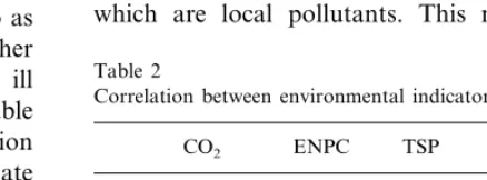
Table 2 presents the correlation between the environmental indicators relating to air pollution. CO2 emissions and ENPC are noted to have a very high positive correlation, while ENPC and CO2 emissions have a weak negative relationship with the emission levels of SO2, TSP and NOx, which are local pollutants. This may be a bit
Table 2
Correlation between environmental indicators (air pollution) TSP
CO2 ENPC SO2 NOx
CO2 1.0
1.0 0.8909 ENPC
TSP −0.2871 −0.3193 1.0
1.0 0.8905
−0.2648
−0.2176 SO2
−0.1060 −0.1451 0.8216 0.8677 1.0 NOx
6There exist alternative data sources for the variables used
in this paper. For example, the World Resources Institute (WRI) provides data on the environment, health and the economy (http://www.wri.org/wri/facts/data-tables.html). WRI data on air pollution is very similar to the kind we use as it is available for a few years, but not over time. The data on water pollution is of better quality in our current source (i.e. World Development Indicators, 1998) compared with that of the WRI. Further, WRI data for water pollution is for differ-ent years for differdiffer-ent countries, with a time span difference of up to 13 years in some cases. Such disparate data would not lend itself to cross-country comparisons, as we require in this study.
7We would like to thank an anonymous referee for bringing
this to our attention.
8The Gini coefficient does have some limitations as a
L.Gangadharan,M.R.Valenzuela/Ecological Economics36 (2001) 513 – 531
522
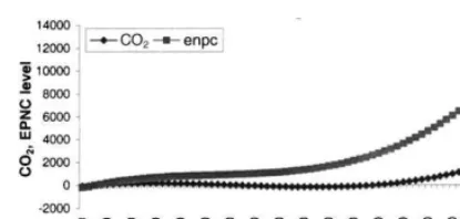
Fig. 1. Estimated relationship between GNP and CO2, ENPC
level.
coefficients are jointly significant.
Fig. 1 shows how CO2 emissions and ENPC levels change with increasing per capita income. At income levels below $5000, environmental stress is seen to increase with energy use increasing much more than carbon dioxide emissions. These emis-sion levels peak at around the $6000 mark, after which energy use plateaus while CO2 emissions decrease until income levels reach $18 000. After this critical income point, rapid rates of increase in energy use and CO2 emission levels are observed. These results contrast with the standard EKC curve in that we do not find an inverted-U curve.10 Rather, we find that the curve is a flattened inverse-S shaped curve where the slope is mostly positive everywhere, except for the inflection point where the slope is zero. The inverse-S shape is observed for both CO2and ENPC variables, with ENPC levels showing larger rates of change over the income scale, that is, the CO2curve is flatter and less variable.
The results imply that we can partition the environmental stress experience of countries into distinct phases. During the first phase when per capita incomes are low, environmental stress is shown to increase but at a diminishing rate. During the second phase when per capita incomes are higher, environmental stress levels appear con-trolled and no increases are observed. The third phase occurs at extremely high incomes when emissions increase again and escalate rapidly. This implies that the impact of income on the environ-ment is more significant at the extreme ends of the income scale. In particular, the results show that very low and very high-income countries tend to experience increasing stress levels in their environ-mental conditions, while there is relatively little change in the environmental stress levels for the middle-income countries.
The results further show that population density level and levels of urbanisation are both positively related to environmental stress while the level of income inequality is inversely related to environ-mental quality. Hence, as a country gets more surprising, as we would expect that a rise in energy
consumption would be accompanied by a rise in pollutant emissions. Suri and Chapman (1998) explain this seemingly inconsistent result by sug-gesting that it is possible for energy consumption to keep rising but for emission levels of local pollutants to fall, as would be the case when end-of-pipe technology like scrubbers are used to reduce local pollutants. As the existing policies to abate local pollution often concentrate on end-of-pipe methods and not on reducing energy consump-tion or emission levels, it should not surprising that energy use and CO2 emissions are not being re-duced along with reductions in the levels of local pollutants.
5. Results
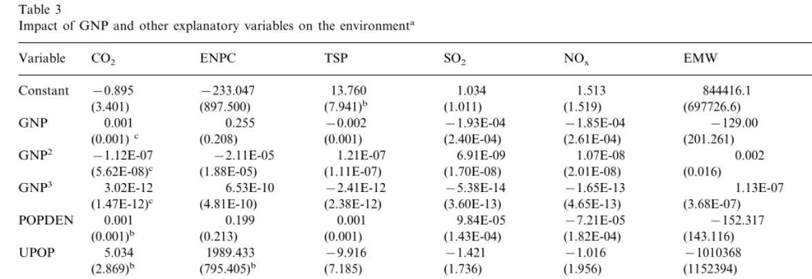
Table 3 presents results from the estimation of the environmental equation (Eq. (2)). It is seen that per capita income, population density, country’s level of urbanisation, inequality in the distribution of income as well as level of education exert significant influences on a country’s level of envi-ronmental stress. The results are particularly strong when CO2 emissions and ENPC are used as the dependent variables. In the case of CO2, we find that when all other influences are taken to be constant, a $1000 increase in per capita GNP increases the per capita CO2 emission level by 1 metric ton. For ENPC, a 255 kg in oil equivalent increase in energy use results from a $1000 increase in per capita GNP.9 The F-test shows that the
10We do not find an inverted-U shaped relationship
be-tween income and any of the pollutants. In the literature, the EKC relationship is supported for pollutants like SO2 and
NOx, but not always for CO2, which is usually seen to increase
over income.
9The coefficients do not come out to be statistically
signifi-cant for ENPC, however, the sign of the income coefficients are very similar to the signs of the income coefficients for CO2
L
.
Gangadharan
,
M
.
R
.
Valenzuela
/
Ecological
Economics
36
(2001)
513
–
531
523
Table 3
Impact of GNP and other explanatory variables on the environmenta
SO2 NOx EMW DEFRTE
CO2
Variable ENPC TSP
844416.1
1.034 1.513
13.760
Constant −0.895 −233.047 0.485, 0.651
(1.011) (7.941)b
(897.500) (697726.6)
(3.401) (1.519)
0.001 −0.002
GNP 0.255 −1.93E-04 −1.85E-04 −129.00 −4.05E-05
(201.261)
(0.001)c (0.208) (0.001) (2.40E-04) (2.61E-04) (2.33E-04)
−2.11E-05 6.91E-09
−1.12E-07
GNP2 1.21E-07 1.07E-08 0.002 −9.46E-10,
(0.016)
(2.01E-08) 1.52E-08
(1.88E-05) (1.70E-08)
(5.62E-08)c (1.11E-07)
−5.38E-14
−2.41E-12 −1.65E-13
6.53E-10 1.13E-07
3.02E-12
GNP3 6.71E-14,
3.12E-13 (3.68E-07)
(2.38E-12) (4.65E-13)
(4.81E-10)
(1.47E-12)c (3.60E-13)
0.199 9.84E-05
0.001
POPDEN 0.001 −7.21E-05 −152.317 −5.45E-05,
(143.116)
(1.82E-04) 1.20E-04
(0.213) (1.43E-04)
(0.001)b (0.001)
−9.916 1989.433
5.034 −1.421
UPOP −1.016 −1010368 0.201, 1.288
(1.956)
(795.405)b (1.736) (1152394)
(2.869)b (7.185)
GINI −0.090 −36.024 0.020 0.017 0.011 11058.34 0.018, 0.015
(0.021) (0.096)
(14.988)b (0.024)
(0.059) (14480.17)
6086.675
0.010 0.002
0.012 −0.008, 0.008
18.411
EDU 0.034
(0.016) (0.011)
(0.046) (7135.055)
(0.034) (7.757)b
4.44 6.96 0.71 0.53 1.08 2.45
F-test 0.83
aFigures in parenthesis indicate robust S.E. bSignificant at 10% level.
L.Gangadharan,M.R.Valenzuela/Ecological Economics36 (2001) 513 – 531
524
crowded (more people on a fixed area of land), the higher will be their CO2emissions and per capita energy use. This can be due to the fact that as population density increases, there is increasing pressure to use the existing land more intensively. The creation of multi-storey residential and com-mercial buildings in high population density coun-tries is a good example of this problem. Lifestyle adjustments for residents in these countries imply more energy consumption and this leads to abnor-mally high levels of CO2emissions. Singapore is a case in point; its population density in 1996 was 4990 persons per km2
and the commercial energy use was 7162 kg of oil equivalent per capita. In contrast, the corresponding average levels for our sample of 51 countries are 206 and 2850, respec-tively. Clearly, the high population density in Singapore exerts a major influence on its extremely high level of energy use. Further, the percentage of population living in urban areas (UPOP) impacts positively on the levels of CO2 and ENPC, with emissions rising as urban population increases.
We observe a positive coefficient for the educa-tion variable (EDU), which runs counter to expec-tations. The results show that higher levels of education aggravate, rather than improve, environ-mental conditions. On the other hand, any im-provement in the inequalities between the rich and the poor is found to be detrimental to the environ-ment. While counter intuitive in the first instance, this makes empirical sense because a move towards more equal standards of living implies more people are able to afford the use of electricity, cars and other luxuries — which leads to increased energy use.11 For such a cross-section of countries, the
explanatory power of these two models is fairly high (adjusted R2
=67% for CO2 and 79% for ENPC).
Eq. (2) was also estimated using data on other specific pollutants such as TSP, SO2, NOx, EMW and DEFRTE. The magnitude and signs of the estimated coefficients are very sensitive to the pollutant used, and are very unstable. Further, the explanatory power of the models are greatly re-duced withF-test results simultaneously indicating inappropriate models. We note that many environ-mental studies used CO2 and ENPC precisely because the data on these variables are well devel-oped. Also, we note here that trend results are similar for CO2and ENPC because CO2is a major component of ENPC. As seen in Table 2, these two environmental stress variables have a high and positive correlation between them.
5.1. Impact on health
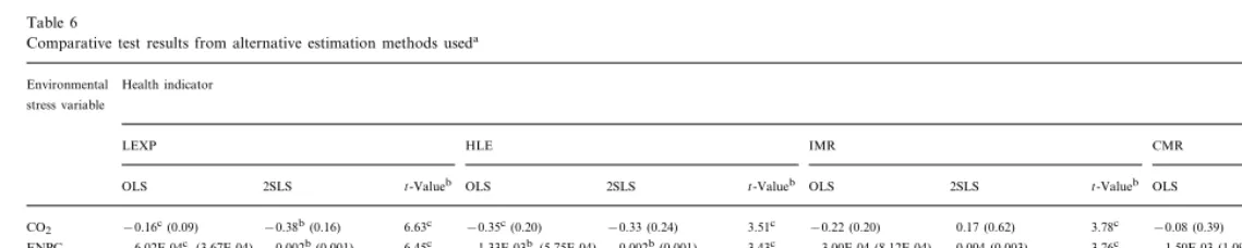
Results of the two-stage least squares (2SLS) estimation of Eq. (3) are presented in Tables 4 and 5. In these estimations, we use alternative indicators of a population’s health status — namely, life expectancy (LEXP), healthy life expectancy (HLE), infant mortality rate (IMR) and child mortality rate (CMR) — and treat the environmental stress variable as endogenous. We find that if we ignore the potential endogeniety of the environmental variables, the results obtained are inconsistent. The Davidson and MacKinnon (1993) augmented re-gression test shows that the null hypothesis of an exogenous environmental stress variable is strongly rejected for all the alternative types of pollutants.12 Table 6 presents the coefficients of the environmen-tal stress variables for the different health indica-tors and compares the OLS and the 2SLS estimates. The coefficients obtained from the 2SLS estimation have signs in the expected direction and the magni-tudes are larger compared with the coefficients from the OLS estimation. This implies that the impact of the environmental stress variable on
11This issue has been analysed in greater detail in Torras and
Boyce (1998), Scruggs (1998) with mixed results. While Torras and Boyce (1998) find that more equitable distributions of income and power tend to result in better environmental quality, Scruggs (1998) shows that equality does not necessarily lead to lower environmental degradation. Magnani (2000) finds that higher levels of income would increase environmental quality provided the negative effect of production of goods and services on pollution levels is more than counterbalanced by the positive effect of growth on the demand for pollution abatement policy. The demand for environmental quality will be affected by inequality levels in the country. As the level of per capita income increases above a critical level, income equality becomes posi-tively correlated with environmental protection; however, be-yond a certain threshold level of income, the correlation between income and environmental protection turns negative.
12The augmented regression is formed by including the
L
.
Gangadharan
,
M
.
R
.
Valenzuela
/
Ecological
Economics
36
(2001)
513
–
531
525
Table 4
Impact of GNP and environment on health: with LEXP and HLE as dependent variablesa
SO2 NOx EMW DEFRTE
Variable CO2 ENPC TSP
(A)Dependent6ariable:life expectancy
62.728 (6.948)b 65.456 (12.590)b 63.381 (5.336)b 58.002 (3.962)b
Constant 57.228 (3.597)b 53.078 (3.250)b 62.143 (5.048)b
−4.152 (5.439) −4.220E-06 (0.470E-06)c −1.803 (3.430)c
−5.144 (5.156)
−0.623 (0.440)
Environmental −0.380 (0.156)b −0.002 (0.001)b
stress variable
3.3E-04 (1.2E-04)b 4.6E-04 (1.4E-04)b 5.01E-04 (1.1E-04)b 4.0E-04 (8.7E-05)b
0.001 (1.6E-04)c
GNP 0.001 (9.3E-05)b 4.1E-04 (7.4E-05)b
0.063 (0.069) 0.087 (0.081)
0.056 (0.104) 0.110 (0.082)
0.095 (0.062)
IMM 0.064 (0.038)c 0.091 (0.033)b
0.012 (0.009)
0.009 (0.004)b 0.013 (0.004)b 0.006 (0.005) 0.005 (0.007) 0.007 (0.004)c −0.001 (0.017)
DOC
−0.004 (0.040)
0.012 (0.022) 0.030 (0.023) 0.008 (0.022) 0.016 (0.021) 0.006 (0.025) 0.002 (0.041)
EDU
−3.737 (4.363) 3.664 (4.506)
−4.054 (6.700)
−5.541 (5.614)
UPOP 3.846 (2.813) 4.932 (3.301) −5.383 (4.526)
9.40 9.43 12.59 21.61
17.27
F-test 23.60 16.16
(B)Dependent6ariable:healthy life expectancy
47.126 (9.874)b 41.164 (6.873)b
37.139 (5.767) 44.883 (8.480)b 47.426 (10.820)b 52.610 (20.266)b
40.236 (6.759)b
Constant
−0.326 (0.237) −0.002b(00.001) −7.256 (7.622) −6.626 (8.987) −5.890E-06c(3.690E-06) 0.320 (4.680)
Environmental −0.603 (0.627)
stress variable
3.053E-04 (1.807E-04)c 5.029E-04 (2.108E-04)b 5.604E-04 (1.665E-04)b 4.652E-04 (1.564E-04)b
7.393E-04 (1.678E-04)b
GNP 0.001 (1.357E-04)b 4.352E-04 (1.115E-04)b
0.146 (0.123) 0.112 (0.099)
0.120 (0.172) 0.196 (0.138)
IMM 0.126 (0.070)c 0.146 (0.061)b 0.157 (0.097)c
0.028 (0.016)c
0.022 (0.008)b 0.025 (0.006)b 0.019 (0.009)b 0.017 (0.011) 0.020 (0.009)c 0.021 (0.026)
DOC
−0.004 (0.048) 0.014 (0.039)
−0.020 (0.070)
0.012 (0.042) 0.004 (0.038)
EDU 0.008 (0.039) 0.023 (0.037)
−4.771 (10.689)
6.504 (3.639)c 7.176 (3.348)b −2.234 (7.330) −5.738 (8.015) −3.463 (6.259) 4.662 (4.797)
UPOP
7.72 7.14 9.43 17.97
19.50
F-test 18.16 14.11
aFigures in parenthesis indicate robust S.E. bSignificant at 5% level.
L
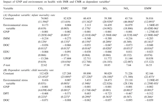
Impact of GNP and environment on health: with IMR and CMR as dependent variablesa
EMW
Variable CO2 ENPC TSP SO2 NOx DEFRTE
(A)Dependent6ariable:infant mortality rate
59.308
74.065 82.829 56.816 75.416
Constant 60.419 45.716
(15.342)b (46.084)b (12.086)b
(13.419)
(11.594)b (20.929)b (12.095)b
2.113 16.439 16.079 1.540E-05 12.889
0.173
Environmental stress 0.004
variable (0.619) (0.003) (1.178)c (14.902) (18.806) (8.420E-06)c (10.253)
−1.270E-03
−0.001 −0.001 −0.001
−0.001
GNP −0.002 −0.001
(3.391E-04)b
(3.586E-04)c (4.523E-04)b
(2.181E-04)b (3.580E-04)b
(0.001)b
EDU 0.011 −0.023 0.034
(0.074)
(0.071) (0.133)
(0.066) (0.064) (0.066) (0.132)
−17.604 11.772
−13.266
UPOP 12.711 11.144 10.838 −24.073
(15.122)
(22.007) (16.440)
(10.654)c (16.183)
(9.619) (12.768)
22.62 17.98 17.64 7.64 16.53 13.39
F-test 10.85
(B)Dependent6ariable:child mortality rate
113.820
(23.089)b (27.228)b (71.380) (22.437)c
(21.052)b (21.322)b
0.416
Environmental stress 0.007 3.433 24.473 23.110 2.190E-05 17.854
(15.862)
(3.176E-04)b (0.001)b
(0.001)b
UPOP −29.605 12.990
(19.265) (33.370) (24.261)
(15.172)c
(13.364)c (24.349) (21.196)
10.61 10.82
17.97 13.91 11.99 6.44 5.36
F-test
aFigures in parenthesis indicate robust S.E. bSignificant at 5% level.
L
.
Gangadharan
,
M
.
R
.
Valenzuela
/
Ecological
Economics
36
(2001)
513
–
531
527
Table 6
Comparative test results from alternative estimation methods useda
Health indicator Environmental
stress variable
CMR IMR
LEXP HLE
t-Valueb OLS 2SLS
OLS 2SLS t-Valueb OLS 2SLS t-Valueb OLS 2SLS t-Valueb
3.51c −0.22 (0.20) 0.17 (0.62) 3.78c −0.08 (0.39)
−0.35c(0.20) 0.42 (0.85)
CO2 −0.16c(0.09) −0.38b(0.16) 6.63c −0.33 (0.24) 4.19c
−6.02E-04c(3.67E-04) −0.002b(0.001) 6.45c −0.002b(0.001) 3.43c 3.00E-04 (8.12E-04) 0.004 (0.003) 3.76c 1.50E-03 (1.09E-03) 0.007c(0.005) 4.03c
ENPC −1.33E-03b(5.75E-04)
0.42 (0.33) −7.26 (7.62) 3.81c 0.53 (1.11) 16.44 (14.90) 3.56c 2.34E-03 (1.40) 24.47 (22.83) 4.06c
−5.14 (5.16)
SO2 0.21 (0.24) 8.35c
4.01c 0.31 (0.98) 16.08 (18.81) 3.62c −0.19 (1.35) 23.11 (28.13)
−6.63 (8.99) 4.13c
8.48c 0.46 (0.31)
NOx 0.28 (0.19) −4.15 (5.44)
−0.60 (0.63)
0.02 (0.07) −0.62 (0.44) 8.45c 0.10 (0.10) 3.74c 0.33 (0.37) 2.11c(1.18) 3.45c 0.34 (0.53) 3.43c(1.95) 3.96c
TSP
3.53c
EMW 6.86E-08 (4.58E-07) −4.22E-06c(2.47E-06) 6.98c 3.45E-07 (5.99E-07) −5.89E-06c(3.69E-06) 1.17E-06 (1.53E-06) 1.54E-05c(8.42E-06) 3.56c 1.20E-06 (2.11E-06) 2.19E-05c(1.25E-05) 4.21c
3.43c 0.03 (2.10) 12.89 (10.25) 3.70c −0.27 (3.08) 17.85 (15.86)
0.32 (4.68) 4.29c
−0.16 (0.77)
DEFRTE −0.25 (0.44) −1.80c(3.43) 7.46c
L.Gangadharan,M.R.Valenzuela/Ecological Economics36 (2001) 513 – 531
528
health is bigger when we take the endogeniety into account. The t-statistic from the Davidson – Mackinnon augmented regression test for exo-geneity shows that the null hypothesis of exogeneity is rejected at the 5% significance level.
Panel A in Table 4 presents the results when life expectancy is the health indicator used. In general, the environmental stress variables have the correct sign (negative) and are significant for certain pollutants such as CO2, EMW, ENPC and DEFRTE.13 GNP is always significant and increases in income levels lead to an increase in life expectancy. The level of immunisation (IMM) is seen to increase life expectancy when the pollutant used is CO2 or ENPC. Education
level (EDU) does not seem to be significant for improving health. The availability of doctors (DOC) as a proportion of the population has a significant impact on improving life expectancy, particularly for the CO2, ENPC and EMW pol-lutants. When the health indicator used is healthy life expectancy (panel B of Table 4), the results are similar. The availability of doctors increases healthy life expectancy significantly; the absolute impact (measured by size of the coefficients) of this variable is also greater with HLE, as the dependent variable. The impact of urbanisation (UPOP) on health is large and sig-nificant particularly for HLE as the dependent variable. This positive impact reflects the soci-ety’s benefits from improvements in the provi-sion of better waste disposal and sanitation facilities, which would come with urbanisation.
When infant mortality is taken as the health indicator (panel A of Table 5), we find that in-creases in TSP emissions and water pollutant emissions levels lead to significantly high infant mortality. Coefficients derived from the estima-tion of the model using the child mortality rates are very similar to the infant mortality results (panel B of Table 5). In general, the results
show that income, immunisation rates, access to doctors and urbanisation levels all make large positive and significant impacts on both infant and child mortality rates. Only the education variable fails to make a significant impact on mortality rates.
We also use log linear models to check for robustness of results. Per capita GNP, purchas-ing power parity, is found to be significant in all cases in improving health. Using log TSP, log SO2, log NOx and log EMW as the environmen-tal stress variable, it is found that the coeffi-cients are negative and significant (for log SO2 and log NOx) in explaining health outcomes. Hence, the environmental variable is significant in explaining changes in health levels in a popu-lation. The estimated coefficients for log CO2 and log ENPC, however, have positive coeffi-cients and are significant. This is contrary to what we would expect. We find, therefore, that in some cases the results could be sensitive to the functional form used.14
6. Conclusion and further research
In this paper, we examine the links between health status, income and environmental indica-tors of a country. We first look at the relation-ship between environment and income — the EKC hypothesis. We find that low-income coun-tries cannot simply postpone attending to envi-ronmental concerns in the hope that the environment will eventually improve with in-creased incomes. Health is a significant interven-ing variable and isolating the impact of environment on health is very important, partic-ularly in the context of developing countries. Our results show that the gains in health ob-tained through improved incomes can be negated to a significant extent if the indirect effect of income, acting via the
environ-13The economic relationship between deforestation and
health indicators is a bit ambiguous. As deforestation is an indicator of ecological balance in the country, this could have long-term effects on health, however, the impact in the short term is not very clear.
14Results for log linear models are not presented in the
L.Gangadharan,M.R.Valenzuela/Ecological Economics36 (2001) 513 – 531 529
ment, is ignored. This study thus shows that policy makers who have chosen to pursue rapid growth strategies at the expense of the environ-ment are not delivering the full realisable health gains that can be derived from higher incomes. Also environmental damage is bound to result in health problems for the domestic population. A less healthy labour force will not be able to increase productivity levels, and hence result in lesser income for the economy. Addressing chronic health problems for the population is also costly and will divert valuable resources from income generating investment projects. Clearly, policies for growth must incorporate appropriate programs for protection of the country’s natural environment and this does not have to be at odds with growth and develop-ment targets.
One of the ways this research can be extended is to obtain time series data on environmental indicators and health status for varied countries along the development spectrum. As we are in-terested in different kinds of environmental and health indicators, obtaining data for all these indicators for many years is quite challenging. Most developing countries do not keep records of environmental variables, and this hampers our objective here. However, with the continued improvements in data availability, over time this problem will be reduced and research on this can be encouraged. A second extension is to create a single indicator or index that could cap-ture the overall quality of a country’s physical environment. Such an index would be useful for analysing environmental issues within a country and can also provide important insights for cross-country trends. A third extension would be to study the impact of environmental policies on income or growth in a country and whether it has an impact on the health outcomes. This could help us in understanding whether the pur-suit of pro-environmental policies would have beneficial or adverse effects on growth itself. This could be examined using a three-equation system with income, environmental stress and health being endogenous variables.
Acknowledgements
We would like to thank Pete Summers, three anonymous referees, seminar participants at the Research School of Pacific and Asian Studies, Australian National University, the participants at the Conference of Economists, 1999, Latrobe University and at the Sixth Biennial Meeting of International Society of Ecological Economics, Canberra, 2000, for their comments. We are, however, responsible for all remaining errors. Funding for this research was provided by the Faculty Research Grant Scheme, Faculty of Economics and Commerce, University of Mel-bourne.
Appendix A. Countries included in the study.
L.Gangadharan,M.R.Valenzuela/Ecological Economics36 (2001) 513 – 531
Agras, J., Chapman, D., 1999. A dynamic approach to the Environmental Kuznets Curve hypothesis. Ecol. Econ. 28, 267 – 277.
Chakrabarti, A., Rao, D.N., 1999. Measuring the impact of policy variables on the burden of disease. Mimeo, Jawaharlal Nehru University.
Cropper, M.L, Simon, N.B., Alberini, A., Sharma, P.K., 1997. The health effects of air pollution in Delhi, India. Policy Research Working Paper 1860, The World Bank. Davidson, R., MacKinnon, J.G., 1993. Estimation and
Infer-ence in Econometrics. Oxford University Press, New York. De Bruyn, S.M., van den Bergh, J.C.J.M., Opschoor, J.B., 1998. Economic growth and emissions: reconsidering the empirical basis of Environmental Kuznets Curve. Ecol. Econ. 25, 161 – 175.
Deininger, K., Squire, L., 1996. Measuring Income Inequality: A New Data-base. World Bank, Washington, DC., mimeographed.
Feachem, R., Kjellstrom, F., Murray, C., Over, M., Phillips, M., 1992. The Health of Adults in the Developing World. Oxford University, Oxford.
Flegg, A.T., 1982. Inequality of income, illiteracy and medical care as determinants of infant mortality in underdeveloped countries. Popul. Stud. 36 (3), 441 – 458.
Galeotti, M., Lanza, A., 1999. Desperately seeking (Environ-mental) Kuznets. Mimeo, International Energy Agency.
Gerdtham, U., Sogaard, J., Andersson, F., Jonsson, B., 1992. An econometric analysis of health care expenditure: a cross-section study of the OECD countries. J. Health Econ. 11, 63 – 84.
Grossman, G., 1995. Pollution and growth. In: Goldin, I., Winters, L.A. (Eds.), The Economics of Sustainable Devel-opment. OECD, Paris, pp. 19 – 46.
Grossman, G., Kreuger, A.B., 1995. Economic growth and the environment. Q. J. Econ. 112, 353 – 377.
Hill, K., King, E., 1992. Women’s education in the third world: an overview. In: King, E., Hill, A.M. (Eds.), Women’s Education in Developing Countries: Barriers, Benefits and Policy. John Hopkins University Press for the World Bank, Baltimore, pp. 1 – 50.
Kakwani, N., 1993. Performance in living standards: an inter-national comparison. J. Dev. Econ. 41 (2), 307 – 336. Kaufmann, R.K., Davidsdottir, B., Garnham, S., Pauly, P.,
1998. The determinants of atmospheric SO2concentrations:
reconsidering the Environmental Kuznets Curve. Ecol. Econ. 25, 209 – 220.
Kuznets, S., 1955. Economic growth and income inequality. Am. Econ. Rev. 45 (1), 1 – 28.
Magnani, E., 2000. The Environmental Kuznets Curve, environ-mental protection policy and income distribution. Ecol. Econ. 32 (3), 431 – 443.
Mellington, N., Cameron, L., 1999. Female education and child mortality in Indonesia. Bull. Indonesian Stud. 35 (3), 115 – 144.
Munasinghe, M., 1999. Is environmental degradation an in-evitable consequence of economic growth: tunneling through the Environmental Kuznets Curve. Ecol. Econ. 29, 89 – 109.
Panayotou, T., 1993. Empirical tests and policy analysis of environmental degradation at different stages of economic development. Working Paper, Technology and Environ-ment Programme, International Labour Office, Geneva. Parpel, F., Pillai, V., 1986. Patterns and determinants of infant
mortality in developing nations, 1950 – 1975. Demography 23 (4), 525 – 542.
Preston, S., 1980. Mortality declines in less developed countries. In: Easterlin, R. (Ed.), Population and Economic Change in Developing Countries. The University of Chicago, Chicago, pp. 289 – 360.
Pritchett, L., Summers, L.H., 1996. Wealthier is healthier. J. Hum. Resour. XXXI (4), 841 – 868.
Scruggs, L., 1998. Political and economic inequality and the environment. Ecol. Econ. 26 (3), 259 – 275.
Selden, T.M., Song, D., 1994. Environmental quality and development: is there a Kuznets Curve for air pollution emissions. J. Environ. Econ. Manage. 27 (2), 147 – 162. Subbarao, K., Raney, L., 1995. Social gains from female
education: a cross-national study. Econ. Dev. Cult. Change 44 (1), 105 – 128.
L.Gangadharan,M.R.Valenzuela/Ecological Economics36 (2001) 513 – 531 531
Torras, M., Boyce, J.K., 1998. Income, inequality and pollu-tion: a reassessment of the Environmental Kuznets Curve. Ecol. Econ. 25, 147 – 160.
UNICEF, 1991 and 1992. The State of the World’s Children.
Oxford University Press, Oxford.
World Bank, 1992. World Development Report 1992: Devel-opment and the Environment. Oxford University Press, New York.