www.elsevier.com / locate / econbase
Small sample properties of the conditional least squares
estimator in SETAR models
*
George Kapetanios
National Institute of Economic and Social Research, Smith Square, 2 Dean Trench Str., London SW1P 3HE, UK
Received 30 April 1999; received in revised form 2 February 2000; accepted 25 May 2000
Abstract
This note considers the small sample performance of the conditional least squares estimator of the threshold parameters in nonlinear threshold and particularly self exciting threshold autoregressive (SETAR) models. It is shown that despite the superconsistency of the threshold parameter estimates the estimator performs poorly in samples of sizes usually encountered in macroeconomics. 2000 Elsevier Science S.A. All rights reserved.
Keywords: Threshold models; SETAR models; Monte Carlo; Superconsistency
JEL classification: C13; C15; C32
1. Introduction
The investigation of nonlinearity in macroeconomic series has attracted considerable attention recently. The class of threshold autoregressive models introduced by Tong (1978) and Tong and Lim (1980) provides a widely used framework for such investigation. The theoretical appeal and relative computational tractability are the major reasons for its use.
This note considers the small sample performance of the conditional least squares estimator in threshold and particularly SETAR models with particular focus on the threshold parameter estimator. It is well known that under certain regularity conditions, this estimator is superconsistent (see Chan (1993)). However, we find that despite this theoretical property, the estimator performs poorly in samples of sizes usually encountered in macroeconomics.
*Tel.:144-207-2227-665; fax: 144-207-6541-900. E-mail address: [email protected] (G. Kapetanios).
2. Theory
We consider the following self exciting threshold autoregressive (SETAR) model
yt5fj,01fj,1yt211 ? ? ? 1fj, pyt2p1s ej t, j51, . . . ,m, t5p, . . . ,T, sj.0 (1)
The model has m regimes. The process is in regime j if rj21#yt2d,r where d is an integer valuedj
delay parameter. r05 2 `and rm5 `. hr . . . r1 m21jis a strictly increasing sequence of parameters to be estimated.et is an i.i.d. zero mean process with unit variance. For simplicity, throughout this paper, we will assume thatet has a standard normal distribution. This model will be denoted as SETAR(m, p,
1
d ). The number of regimes, m, and the delay parameter, d, are assumed known in our setup . We note
that p is the true lag order for all the m regimes. Estimation is carried out by constructing a grid of possible values for r , jj 51, . . . ,m21 and running the regressions
yj5Xjfj1ej, j51, . . . ,m (2)
for each point in the threshold parameter grid, where y and X are a vector and matrix, respectively,j j containing the observations for regime j.fjandejare the coefficient and error vectors for regime j. In matrix notation, yj5( y , y , . . . , y )j j j 9, Xj5(x , . . . ,x )j j 9, xj 5( yj21, yj22, . . . , yj2p)9, fj5
1 2 Tj 1 Tj i i i i
(fj,1, . . . ,fj, p)9 ej5(ej , . . . ,ej )9 and hj , j , . . . , j1 2 Tj are the time indices of the observations
1 Tj j
belonging to regime j, j51, . . . ,m. The grid point which minimises the sum of squared residuals from the m regressions is adopted as the estimate for the threshold parameters. Chan (1993) proves that under geometric ergodicity and some other regularity conditions the threshold parameters are consistent, tend to their true value at rate T, and suitably normalised follow asymptotically a
21 / 2
compound Poisson process. The other parameters of the model are T consistent and are asymptotically normally distributed. To the best of our knowledge investigation of the small samples properties of the parameter estimates and particularly the threshold parameter estimates has not been undertaken. A Monte Carlo investigation is carried out in the next section.
3. Monte Carlo investigation
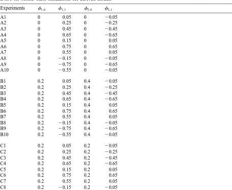
We aim to investigate the properties of the conditional least squares estimator for a variety of parametric setups so as to minimise the risk of drawing invalid conclusions due to idiosyncracies of a particular model design. Preliminary investigation suggested that the results obtained for SETAR models of two regimes readily extend to models with three regimes. SETAR models with more regimes have not been considered due to excessive computational cost. The same conclusion was reached for models with more than one lags. We therefore provide the results of an extensive investigation on SETAR(2,1,1) models. It is likely that the performance of the conditional least squares estimator will depend on the magnitude and signs of the coefficients fj,i, j51, 2, i50, 1. The set of DGPs we therefore consider is given in Table 1.
1
Table 1
DGPs for Monte Carlo simulations for SETAR models
since f1,1.0, f2,1.0 (Experiments A5–A7, B5–B7 and C5–C7). Finally, within each subset of experiments we vary both the magnitude of the difference of the autoregressive coefficient between the two regimes as well as the absolute magnitude of the autoregressive coefficient.
The threshold parameter, r, is estimated by grid search. The grid points are obtained using the quantiles of the sample under investigation as suggested by Tsay (1989) and Tong and Lim (1980), In particular 21 equally spaced quantiles are used starting from the 10% quantile and ending at the 90% quantile, i.e. we use the 10%, 14%, 18% . . . 86%, 90% quantiles of the sample. The sample size, T, takes the values 100, 200 and 400. The error terms are constructed to be zero mean normal variates. For each replication a sample of size T1200 is initially generated. The first 200 observations of each
2
sample are discarded to minimise the effect of initial conditions . For each of the DGPs and for each
T, 1000 replications are carried out. The bias and the mean square error of the estimated parameters
over the 1000 replications for all the experiments are given in Tables 2–4.
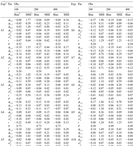
The coefficients of the SETAR models do not exhibit significant bias and the bias that appears is reduced significantly when the sample size is increased. The mean square error of the estimators behaves similarly. The major exception to this finding is the behaviour of the estimators of the constant terms which exhibit bigger biases than the other coefficients and large mean square errors. Nevertheless, even these estimators improve significantly when the sample size is increased.
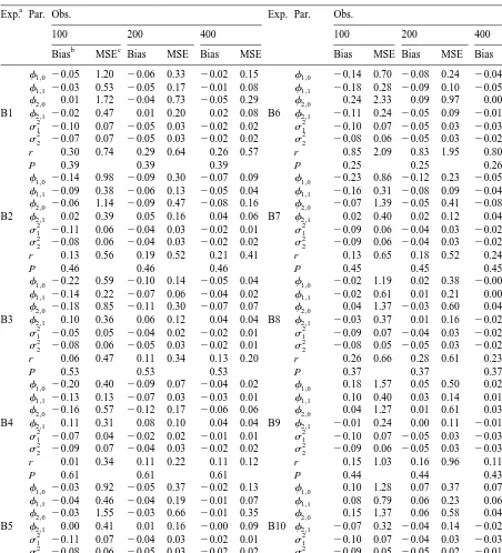
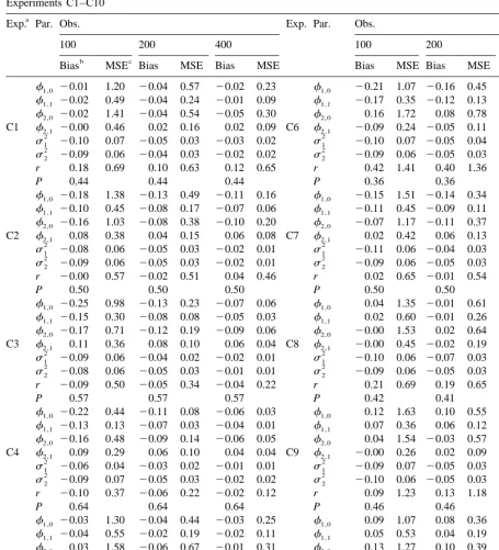
The estimator of the threshold parameter exhibits large biases in a number of cases, especially when the constant terms in the model are different from zero. Examples include experiments B1, B5, B6 and their counterparts in the set of experiments C. The biases tend to be reduced for larger sample sizes but not uniformly over the experiments. Additionally, in a number of experiments the MSEs of the estimator remain large even for 400 observations in contrast to the MSE of the other parameter estimators. It is worthwhile to note that whereas the MSE of the threshold parameter estimator is comparable to the MSEs of the other parameter estimators in small sample sizes (e.g. T5100) it is always larger than them for T5400, sometimes by a factor of ten. It is clear that the performance of the estimator improves much more as the sample size increases when the autoregressive parameters in the two regimes differ significantly. Further, when the autoregressive parameters are large in absolute values then the performance of the threshold parameter estimator deteriorates always in terms of bias and in most cases in terms of MSE.
Overall, we conclude that despite the superconsistency result mentioned earlier, the threshold parameter estimator behaves poorly in small samples, relatively to the other parameter estimators.
4. The conditional sum of squares function
In order to investigate further this result we analyse the conditional sum of squares (CSS) of the models as a function of the threshold parameters. The CSS function is defined as
m
CSS(r , . . . ,r1 m21;f)5
O
ej(r , . . . ,r1 m21;f)9ej(r , . . . ,r1 m21;f)j51
2
Table 2
Bias MSE Bias MSE Bias MSE Bias MSE Bias MSE Bias MSE
f1,0 20.08 1.77 20.04 0.69 20.04 0.34 f1,0 20.37 1.90 20.19 0.60 20.13 0.27
Exp.: Experiment; Par.: Parameters; Obs.: Sample size; P: Proportion of observations in lower regime; MSE: Mean square error.
b N n n
ˆ ˆ
The bias is given by 1 /N on51a 2 a wherea is the relevant parameter estimate for replication n anda is the true value of the relevant parameter and N51000.
c N n 2
Table 3
Bias MSE Bias MSE Bias MSE Bias MSE Bias MSE Bias MSE
f1,0 20.05 1.20 20.06 0.33 20.02 0.15 f1,0 20.14 0.70 20.08 0.24 20.04 0.09
Exp.: Experiment; Par.: Parameters; Obs.: Sample size; P: Proportion of observations in lower regime; MSE: Mean square error.
b N n n
ˆ ˆ
The bias is given by 1 /N on51a 2 a wherea is the relevant parameter estimate for replication n anda is the true value of the relevant parameter and N51000.
c N n 2
Table 4
Bias MSE Bias MSE Bias MSE Bias MSE Bias MSE Bias MSE
f1,0 20.01 1.20 20.04 0.57 20.02 0.23 f1,0 20.21 1.07 20.16 0.45 20.11 0.18
Exp.: Experiment; Par.: Parameters; Obs.: Sample size; P: Proportion of observations in lower regime; MSE: Mean square error.
b N n n
ˆ ˆ
The bias is given by 1 /N on51a 2 a wherea is the relevant parameter estimate for replication n anda is the true value of the relevant parameter and N51000.
c N n 2
where ej(r , . . . ,r1 m21; f)5yj2Xjfj is the error vector for regime j implicitly defined in (2) and
9
9
f5(f1, . . . ,fm)9. Note that we modify slightly our notation to explicitly state the dependence of the error vectors on the threshold parameters and the fact that we take the coefficients,f, as given. To simplify notation we supress the dependence of the above quantities on the sample size, T. We would like to obtain the expected value of CSS(r;f) for the SETAR(2,1,1) model we are investigating over a grid of possible values of r. We resort to simulation techniques to obtain an estimate of that expectation. The simulation estimator is given by
N 2
2 1 n n
]
CSS(r;f)5
O O
ej(r;f)9ej(r;f) (3)Nn51 j51
n n n n n
where ej(r; f)5yj 2Xjfj. y and X , jj j 51,2 are obtained from simulated samples constructed using the DGPs given in Table 1. N is the number of replications. The parameter values, f, used to
2 2 p
evaluate CSS(r;f) are the true parameter values from Table 1. It is clear that CSS(r;f)→E(CSS(r;
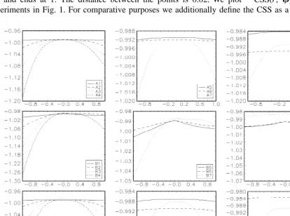
f)) as N→`. We set N52000, T5100 and use a grid of equally spaced values for r which starts at 2
21 and ends at 1. The distance between the points is 0.02. We plot 2CSS(r; f) over r for all experiments in Fig. 1. For comparative purposes we additionally define the CSS as a function of one
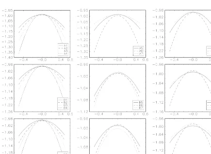
of the coefficients which we choose to bef1,1. In the notation we introduced above this is denoted as CSS(f1,1; r, f0,1, f2,0, f2,1). We estimate the expectation of CSS(f1,1; r, f0,1, f2,0, f2,1) using a similar estimator to the one given in (3). Once again the parameters used to generate the simulated samples are taken from Table 1 and N52000, T5100. Denoting the true value of f1,1 for
0 0
experiment i by if1,1, the grid used for f1,1 and experiment i is given by Gi5hif1,120.5,
0 0 0 0 0 0
f 20.48, . . . , f 20.02, f , f 10.02, . . . , f 10.48, f 10.5j. We plot
i 1,1 i 1,1 i 1,1 i 1,1 i 1,1 i 1,1
2
2CSS(f1,1; r, f0,1, f2,0, f2,1) over Gi for all experiments in Fig. 2.
The plots reveal the reason for the poor performance of the threshold parameter estimator. Whereas
2 2
CSS(f1,1; r, f0,1, f2,0, f2,1) is a smooth quadratic function of f1,1, CSS(r;f)) is less well behaved.2 In general, when the autoregressive parameters do not differ significantly between regimes CSS(r;f)) is very flat exhibiting variation less than 0.001 throughout the grid of r. When the autoregressive parameters differ significantly the variation increases dramatically. When there is a nonzero constant
2
term which differs between regimes, CSS(r;f) exhibits a kink at the true threshold parameter value. The appearance of the kink seems to depend more on the fact that the constant is different between
2
regimes and less on the fact that it is non-zero. Finally, in a number of cases, CSS(r;f) is asymmetric
around the true threshold parameter value. The above results do not change when we consider larger
3
sample sizes .
Overall, it is safe to conclude that the nonstandard features of the CSS function with respect to the threshold parameter lie behind the poor performance of the threshold parameter estimator in small samples.
5. Conclusions
This note has investigated the small sample performance of the conditional least square estimator for self exciting threshold autoregressive models. Particular emphasis was placed on the performance of the estimator for the threshold parameters. Despite the superconsistency result for those parameters it is found that the estimator behaves poorly in small samples. This evidence is in accord with the evidence provided by Psaradakis and Sola (1998) on the poor performance on the maximum likelihood estimator for Markov switching models. Clearly nonlinearity poses a challenge for estimation in small samples. Further research should concentrate on whether this phenomenon persists in other classes of threshold models such as STAR models, TAR models with exogenous variables and endogenous threshold autoregressive (EDTAR) models (see Pesaran and Potter, 1997; Kapetanios, 1998).
Acknowledgements
This work has been carried out as part of the author’s Ph.D. thesis. I would like to thank Hashem Pesaran for his help and Gary Koop and Sean Holly for constructive comments.
References
Chan, K.S., 1993. Consistency and limiting distribution of the least squares estimator of a threshold model. Annals of Statistics 21 (1), 520–533.
Kapetanios, G., 1998. Essays on the Econometric Analysis of Threshold Models. University of Cambridge, Ph.D. Thesis. Pesaran, M.H., Potter, S., 1997. A floor and ceiling model of US. output. Journal of Economic Dynamics and Control 21
(4-5), 661–696.
Psaradakis, Z., Sola, M., 1998. Finite-sample properties of the maximum likelihood estimator in autoregressive models with Markov switching. Journal of Econometrics 86, 369–386.
Tong, H., 1978. In: Chen, C.H. (Ed.), On a threshold model, pattern recognition and signal processing. Sijthoff and Noordhoff, Amsterdam.
Tong, H., Lim, K.S., 1980. Threshold autoregression, limit cycles and cyclical data (with discussion). Journal of the Royal Statistical Society, B 42, 245–292.
Tsay, R.S., 1989. Testing and modelling threshold autoregressive processes. Journal of the American Statistical Association 84 (405), 231–240.
3