LAPORAN KEMAJUAN PENELITIAN DOKTOR BARU DANA ITS 2020

(1)

LAPORAN KEMAJUAN

PENELITIAN DOKTOR BARU DANA ITS 2020

Performa Diagram Kontrol Multivariat Dynamic Hotelling's T

²

dalam Memonitor Mixed Quality Characteristics dengan Principal Component

Analysis (PCA)

Tim Peneliti:

Dr. Muhammad Ahsan, S.Si. (Statistika/FSAD) Dr. Muhammad Mashuri M.T. (Statistika/FSAD)

Dr. Hidayatul Khusna S.Si (Statistika/FSAD) Wibawati S.Si., M.Si. (Statistika/FSAD)

DIREKTORAT RISET DAN PENGABDIAN KEPADA MASYARAKAT

Sesuai Surat Perjanjian Pelaksanaan Penelitian No: 861/PKS/ITS/2020

(2)

Daftar Isi

Daftar Isi ... i

Daftar Tabel ... ii

Daftar Gambar ... iii

Daftar Lampiran ... iv

BAB I RINGKASAN ... 1

BAB II HASIL PENELITIAN ... 2

2.1 Latar Belakang Penelitian ... 2

2.2 Tahapan Penelitian ... 3

2.3 Hasil Penelitian Penelitian ... 5

BAB III STATUS LUARAN ... 11

BAB IV KENDALA PELAKSANAAN PENELITIAN ... 12

BAB V RENCANA TAHAPAN SELANJUTNYA ... 13

BAB VI DAFTAR PUSTAKA ... 14

BAB VIII LAMPIRAN ... 15

LAMPIRAN 1 Tabel Daftar Luaran ... 16

(3)

Daftar Tabel

Tabel 2.1 Performa dari diagram kontrol pada data metric berdistribusi Multivariat Normal untuk dua data non-metric dengan  ₁, ₂ =0,3 dan ₃=0, 4

Tabel 2.2 Performa dari diagram kontrol pada Data metric berdistribusi Multivariat Normal untuk dua data non-metric dengan  ₁, ₂ =0,1 dan ₃=0,8

Tabel 2.3 Performa dari diagram kontrol pada data metric berdistribusi Multivariat Normal untuk dua data non-metric dengan  ₁, ₂ =0, 05 dan ₃ =0,9.

Tabel 2.4 Performa dari diagram kontrol pada data metric berdistribusi Multivariat Normal untuk tiga data non-metric dengan  ₁, ₂ =0,3 dan ₃=0, 4

Tabel 2.5 Performa dari diagram kontrol pada data metric berdistribusi Multivariat Normal untuk tiga data non-metric dengan  ₁, ₂ =0,1 dan ₃=0,8

Tabel 2.6 Performa dari diagram kontrol pada data metric berdistribusi Multivariat Normal untuk tiga data non-metric dengan  ₁, ₂ =0, 05 dan ₃ =0,9.

Tabel 2.7 Performa dari diagram kontrol pada data metric berdistribusi Multivariat Normal untuk lima data non-metric dengan  ₁, ₂ =0,3 dan ₃=0, 4

Tabel 2.8 Performa dari diagram kontrol pada Data metric berdistribusi Multivariat Normal untuk lima data non-metric dengan  ₁, ₂=0,1 dan ₃=0,8

Tabel 2.9 Performa dari diagram kontrol pada data metric berdistribusi Multivariat Normal untuk lima data non-metric dengan  ₁, ₂ =0, 05 dan ₃ =0,9.

Tabel 3.1 Status Luaran Wajib Tabel 3.1 Status Luaran Tambahan

(4)

Daftar Gambar

Gambar 2.1 Diagram alir prosedur diagram multivariat berbasis PCA Mix

Gambar 2.2 Diagram alir prosedur evaluasi performa diagram kontrol multivariat berbasis PCA Mix Gambar 2.3 Diagram alir prosedur evaluasi performa diagram kontrol multivariat berbasis PCA Mix untuk deteksi outlier

(5)

Daftar Lampiran

Lampiran 1 Tabel Daftar Luaran Lampiran 2 Luaran Paper untuk Jurnal Lampiran 3 Luaran Paper untuk Conference

(6)

BAB I RINGKASAN

Dua jenis diagram kontrol dikembangkan berdasarkan karakteristik kualitas yang berbeda yaitu diagram kontrol variabel dan atribut. Karakteristik kulaitas ini biasanya dipantau menggunakan prosedur terpisah.

Hanya beberapa penelitian yang berfokus pada pemanfaatan diagram kontrol untuk memantau proses dengan mixed karakteristik kualitas. Studi ini mengembangkan konsep baru dari diagram kontrol berdasarkan pada metode Principal Component Analysis (PCA) mix, yaitu metode PCA yang dapat bersama-sama menangani data kontinu dan kategorikal. Metode Kernel Density Estimation (KDE) digunakan untuk menghitung Dynamic Control Limit. Selanjutnya, performa dari diagram kontrol akan dievaluasi dalam mendeteksi pergeseran proses menggunakan Average Run Length (ARL) dan dalam medeteksi adanya outlier.

Kata kunci: Mixed quality characteristics, Principal Component Analysis, Kernel Density Estimation, Average Run Length.

(7)

Ringkasan penelitian berisi latar belakang penelitian,tujuan dan tahapan metode penelitian, luaran yang ditargetkan, kata kunci

BAB II HASIL PENELITIAN

2.1 Latar Belakang Penelitian

Diagram kontrol multivariat konvensional yang pertama kali dikembangkan adalah Hotelling’s T² dan χ². Diagram kontrol Hotelling T² pertama kali diperkenalkan oleh Hotteling [1]. Akan tetapi, diagram kontrol Hotelling T² tidak sensitif untuk mendeteksi pergeseran yang kecil pada vektor rata-rata. Karena itu, Woodall dan Ncube [2] memperkenalkan diagram kontrol Multivariate Cumulative Sum (MCUSUM) sebagai diagram kontrol alternatif untuk memonitor vektor rata-rata dari suatu karakteristik kualitas.

Disamping MCUSUM, diagram kontrol lain yang dapat memonitor pergeseran proses yang kecil pada vektor rata-rata adalah diagram kontrol Multivariate Exponentially Weighted Moving Average (MEWMA). [3]

mengembangkan diagram kontrol T²berbasis Princial Component Analysis (PCA). Di tahun yang sama Jackson juga mengembangkan diagram kontrol berbasis Independent Principal Componen Score.

Memonitor data metric dan non-metric dalam sebuah proses manufaktur terkadang perlu untuk dilakukan [4]. Sejauh ini, masih sangat sedikit diagram kontrol dikembangkan yang dapat digunakan untuk pengontrolan kualitas pada kedua jenis data tersebut secara bersamaan. Aslam et al. [5] mengusulkan diagram kontrol mixed menggunakan kombinasi prosedur dari

X

dan np untuk memonitor proses dan menemukan bahwa diagram kontrol mixed lebih efisien dibandingkan diagram kontrol konvensional. Aslam et al. [6] mengusulkan dua diagram kontrol mixed berbasis statsitik EWMA dan Hybrid Exponential Weighted Moving Average (HEWMA) dengan mengasumsikan kualitas karakteristiknya berdistribusi normal, kemudian membandingkan perfroma kedua diagram kontrol tersebut dengan diagram kontrol mixed dari Aslam et al. [5]. Performa diagram kontrol mixed berbasis statistik HEWMA mengalahkan performa diagam kontrol mixed EWMA dan diagram kontrol mixed

X

. Khan et al. [7] mengusulkan diagram kontrol mixed dengan mengasumsikan karasteristik kualitasnya berdistribusi Weibull untuk life testing. Akan tertapi, diagram-diagram mixed tersebut hanya untuk kasus univariate yang diperuntukkan untuk memonitor data metric dan non-metric secara bersamaan. Kenyataannya, proses tersebut bisa monitor hanya dengan salah satu jenis diagram kontrol, baik itu diagram variabel untuk data metric maupun diagram atribut untuk data non-metric. Wang et al. [8] mengusulkan diagram berbasis spatial-sign covariance matrix dengan mengkombinasikan standardized ranks dan spatial signs untuk menghitung statistik dari diagram mixed yang diusulkan.

Untuk mengatasi masalah perbedaan jenis data, dengan menggunakan konsep dari PCA Mix akan diusulkan diagram kontrol baru yang diberi nama diagram kontrol PCA Mix. Adapun dalam penentuan batas kontrolnya akan digunakan konsep kernel density estimation (KDE) yang telah terbukti menghasilkan

(8)

2.2 Tahapan Penelitian

Terdapat tiga tahapan dalam penelitian ini yaitu: tahap pengembangan diagram, evaluasi kinerja diagram, dan penerapan diagram. Secara rinci penjelasan untuk tiap tahapan adalah sebagai berikut:

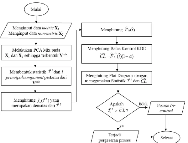
1. Pengembangan diagram control multivariat berbasis PCA Mix

Pada tahapan ini diagram kontrol baru dikembangkan melalui langkah-langkah berikut:

a. Mengidentifikasi sifat-sifat dari statistik T² berbasis PCA Mix yang dikembangkan b. Melakukan perbaikan batas kontrol menggunakan KDE.

c. Melakukan monitoring proses menggunakan statistik mixed seperti pada gambar 4.1.

Gambar 2.1 Diagram alir prosedur diagram multivariat berbasis PCA Mix 2. Evaluasi performa

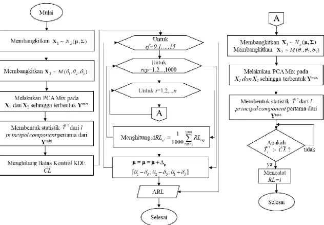
Pada tahapan ini diagram kontrol baru yang telah dikembangkan dievaluasi kinerjanya menggunakan Average Run Length (ARL). Secara detail, langkah-langkah evaluasi kinerja untuk diagram ini adalah sebagai berikut:

Perhitungan ARL0:

(9)

d. Mengulangi langkah a sampai c sebanyak 10000 kali

e. Menghitung ARL0 yang merupakan rata-rata dari run length dari 10000 kali pembangkitan data dalam kondisi in control.

Gambar 2.2 Diagram alir prosedur evaluasi performa diagram kontrol multivariat berbasis PCA Mix Perhitungan ARL1:

a. Membangkitkan data metric berdistribusi Multivariat Normal dan non-metric berdistribusi Multinomial yang telah mengalami pergeseran proses.

b. Menghitung statistik dari diagram kontrol yang diusulkan.

c. Mencatat run length, dinama run length merupakan jumlah observasi sampai terjadi out of control untuk yang pertama kali menggunakan batas kontrol.

d. Mengulangi langkah a sampai c sebanyak 10000 kali

e. Menghitung ARL1 yang merupakan rata-rata dari run length dari 10000 kali pembangkitan.

f. Mengulangi langkah a sampai e dengan berbagai menambahkan pergeseran pada proses.

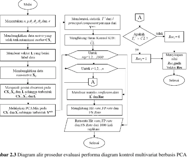
Evaluasi performa untuk deteksi outlier disajikan pada Gambar 2.3

(10)

Gambar 2.3 Diagram alir prosedur evaluasi performa diagram kontrol multivariat berbasis PCA Mix untuk deteksi outlier

2.3 Hasil Penelitian Penelitian

Kasus dua data non-metric

Tabel 2.1 menampilkan performa dari diagram kontrol yang diusulkan untuk memonitor outlier pada dua data non-metric dengan  ₁, ₂ =0,3 dan ₃=0, 4. Terlihat bahwa pada kondisi ini kesalahan deteksi terjadi akibat dari banyaknya observasi yang seharusnya in-control namun dideklarasikan sebagai outlier.

Performa dari diagram kontrol yang diusulkan dalam memonitor dua data non-mertic dengan

1, 2 0,1 dan 3 0,8

  =  = disajikan pada Tabel 2.2. Berbeda dengan kondisi sebelumnya, terlihat bahwa kesalahan deteksi diakibatkan oleh ketidakmampuan diagram kontrol untuk menangkap adanya outlier yang dapat diketahui dari tingginya nilai FN rate. Selanjutnya, untuk performa diagram kontrol ketika memonitor dua data non-metric dengan  ₁, ₂ =0, 05 dan ₃ =0,9ditampilkan pada Tabel 2.3. Pada kondisi ini,

(11)

Tabel 2.1 Performa dari diagram kontrol pada data metric berdistribusi Multivariat Normal untuk dua data non-metric dengan  ₁, ₂ =0,3 dan ₃ =0, 4

ε=5% ε=10%

Hit Rate FN Rate FP Rate Hit Rate FN Rate FP Rate

p=5, l =2 0,96966 0,0000 0,0319 0,95122 0,0002 0,0542

p=5, l =3 0,97353 0,0000 0,0279 0,95445 0,0005 0,0506

p=5, l =4 0,96633 0,0000 0,0355 0,94993 0,0001 0,0556

ε=20% ε=30%

p=5, l =2 0,86096 0,0020 0,1733 0,78931 0,0216 0,2917

p=5, l =3 0,90388 0,0033 0,1193 0,78449 0,0204 0,2991

p=5, l =4 0,88373 0,0034 0,1445 0,79002 0,0230 0,2901

ε=40% ε=50%

p=5, l =2 0,64591 0,0893 0,5306 0,49819 0,2534 0,7502

p=5, l =3 0,64703 0,0860 0,5310 0,50135 0,2661 0,7312

p=5, l =4 0,65355 0,0939 0,5148 0,50137 0,2373 0,7600

Tabel 2.2 Performa dari diagram kontrol pada Data metric berdistribusi Multivariat Normal untuk dua data non-metric dengan  ₁, ₂=0,1 dan ₃ =0,8

ε=5% ε=10%

p=5, l =2 0,99487 0,0132 0,0047 0,99012 0,0260 0,0081

p=5, l =3 0,98997 0,1972 0,0002 0,96837 0,3140 0,0003

p=5, l =4 0,97897 0,2988 0,0064 0,95275 0,4135 0,0066

ε=20% ε=30%

p=5, l =2 0,96786 0,0992 0,0154 0,88818 0,2901 0,0354

p=5, l =3 0,89210 0,5359 0,0009 0,76512 0,7760 0,0030

p=5, l =4 0,86946 0,6205 0,0080 0,74975 0,8068 0,0117

ε=40% ε=50%

p=5, l =2 0,72744 0,5326 0,0992 0,50086 0,7921 0,2062

p=5, l =3 0,63372 0,8995 0,0108 0,50003 0,9693 0,0307

p=5, l =4 0,62190 0,9167 0,0190 0,50082 0,9614 0,0370

(12)

Tabel 2.3 Performa dari diagram kontrol pada data metric berdistribusi Multivariat Normal untuk dua data non-metric dengan  ₁, ₂ =0, 05 dan ₃ =0,9.

ε=5% ε=10%

p=5, l =2 0,97936 0,3600 0,0028 0,94568 0,5218 0,0024

p=5, l =3 0,95731 0,8080 0,0024 0,91529 0,8210 0,0029

p=5, l =4 0,95375 0,8480 0,0041 0,90554 0,9110 0,0037

ε=20% ε=30%

p=5, l =2 0,84812 0,7440 0,0039 0,72375 0,9128 0,0034

p=5, l =3 0,81917 0,8886 0,0039 0,70786 0,9673 0,0028

p=5, l =4 0,81048 0,9301 0,0044 0,70713 0,9621 0,0060

ε=40% ε=50%

p=5, l =2 0,60831 0,9717 0,0050 0,50009 0,9920 0,0078

p=5, l =3 0,60242 0,9892 0,0032 0,50004 0,9889 0,0111

p=5, l =4 0,60167 0,9875 0,0055 0,49978 0,9917 0,0087

Tabel 2.4 Performa dari diagram kontrol pada data metric berdistribusi Multivariat Normal untuk tiga data non-metric dengan  ₁, ₂ =0,3 dan ₃ =0, 4

ε=5% ε=10%

Hit Rate FN Rate FP Rate Hit Rate FN Rate FP Rate

p=5, l =2 0,96961 0,0004 0,0320 0,95411 0,0001 0,0510

p=5, l =3 0,94098 0,0000 0,0621 0,92895 0,0003 0,0789

p=5, l =4 0,94272 0,0000 0,0603 0,91451 0,0000 0,0950

ε=20% ε=30%

p=5, l =2 0,90321 0,0030 0,1202 0,77372 0,0193 0,3150

p=5, l =3 0,81657 0,0005 0,2292 0,71108 0,0106 0,4082

p=5, l =4 0,81361 0,0010 0,2327 0,70425 0,0111 0,4177

ε=40% ε=50%

p=5, l =2 0,62677 0,0711 0,5746 0,49915 0,2422 0,7595

p=5, l =3 0,60148 0,0522 0,6294 0,50158 0,1654 0,8314

p=5, l =4 0,60654 0,0587 0,6167 0,49921 0,2002 0,8014

(13)

diagram kontrol yang diusulkan dalam memonitor tiga data non-metric untuk  ₁, ₂=0,1 dan ₃=0,8 serta  ₁, ₂ =0, 05 dan ₃ =0,9. Sama seperti kasus sebelumnya, pada kasus ini, kesalahan deteksi diakibatkan oleh banyaknya observasi yang gagal dideteksi sebagai outlier. Pada kasus ini juga dapat disimpulkan bahwa penggunaan sedikit principal component memberikan hasil akurasi yang lebih baik.

Selain itu, dapat disimpulkan juga bahwa data non-metric yang memiliki proporsi yang tidak seimbang memberikan tingkat akurasi yang lebih baik.

Tabel 2.5 Performa dari diagram kontrol pada data metric berdistribusi Multivariat Normal untuk tiga data non-metric dengan  ₁, ₂=0,1 dan ₃ =0,8

ε=5% ε=10%

p=5, l =2 0,99409 0,0256 0,0049 0,98687 0,0625 0,0076

p=5, l =3 0,85182 0,0548 0,1531 0,84175 0,1190 0,1626

p=5, l =4 0,96442 0,2608 0,0237 0,93301 0,3925 0,0308

ε=20% ε=30%

p=5, l =2 0,94115 0,1742 0,0300 0,83769 0,3934 0,0633

p=5, l =3 0,80244 0,2704 0,1793 0,72151 0,4766 0,1936

p=5, l =4 0,85371 0,5784 0,0383 0,74692 0,7264 0,0502

ε=40% ε=50%

p=5, l =2 0,67938 0,6334 0,1121 0,50034 0,7424 0,2569

p=5, l =3 0,60897 0,6680 0,2064 0,49729 0,7581 0,2473

p=5, l =4 0,62444 0,7973 0,0944 0,49841 0,8594 0,1438

Tabel 2.6 Performa dari diagram kontrol pada data metric berdistribusi Multivariat Normal untuk tiga data non-metric dengan  ₁, ₂ =0, 05 dan ₃ =0,9.

ε=5% ε=10%

p=5, l =2 0,96109 0,3710 0,0214 0,9189 0,5667 0,0271

p=5, l =3 0,88371 0,4712 0,0976 0,84522 0,6543 0,0993

p=5, l =4 0,93443 0,7830 0,0278 0,88509 0,8596 0,0322

ε=20% ε=30%

p=5, l =2 0,81906 0,7567 0,0370 0,70547 0,8617 0,0514

p=5, l =3 0,76344 0,7958 0,0968 0,66809 0,8776 0,0981

p=5, l =4 0,79227 0,8775 0,0403 0,68634 0,8911 0,0662

ε=40% ε=50%

(14)

Kasus lima data non-metric

Tabel 2.7 menampilkan hasil monitoring outlier pada lima data non-metric dengan

1, 2 0,3 dan 3 0, 4.

  =  = Terlihat bahwa banyaknya observasi yang salah dideteksi sebagai outlier merupakan kesalahan deteksi yang banyak terjadi pada kondisi ini. Performa dari diagram kontrol dalam mendeteksi outlier dengan lima data non-metric dengan  ₁, ₂ =0,1 dan ₃ =0,8 serta

1, 2 0, 05 dan 3 0,9

  =  = masing-masing diberikan pada Tabel 2.8 dan 2.9. Sama sepeti dua kasus sebelumnya, pada kondisi ini, kesalahan deteksi terjadi dikarenakan oleh banyaknya outlier yang gagal dideteksi (FN rate yang tinggi). Secara umum, terlihat bahwa penggunaan principal component yang sedikit mengakibatkan nilai hit rate yang lebih baik. Untuk data non-metric yang hampir seimbang, terlihat bahwa semakin banyak data non-metric yang dianalisis dapat meningkatkan hit rate dari diagram yang diusulkan.

Tabel 2.7 Performa dari diagram kontrol pada data metric berdistribusi Multivariat Normal untuk lima data non-metric dengan  ₁, ₂ =0,3 dan ₃ =0, 4

ε=5% ε=10%

p=5, l=2 0,99097 0,0010 0,0095 0,98861 0,0035 0,0123

p=5, l =3 0,98939 0,0024 0,0110 0,98264 0,0040 0,0188

p=5, l =4 0,98968 0,0016 0,0108 0,98590 0,0051 0,0151

ε=20% ε=30%

p=5, l=2 0,96411 0,0226 0,0394 0,89619 0,0991 0,1058

p=5, l =3 0,95652 0,0252 0,0480 0,87571 0,0956 0,1366

p=5, l =4 0,95204 0,0249 0,0537 0,87924 0,1079 0,1263

ε=40% ε=50%

p=5, l=2 0,73821 0,2665 0,2587 0,50111 0,5183 0,4794

p=5, l =3 0,72134 0,2432 0,3023 0,49897 0,5168 0,4852

p=5, l =4 0,72961 0,2916 0,2562 0,49995 0,5059 0,4942

(15)

Tabel 2.8 Performa dari diagram kontrol pada Data metric berdistribusi Multivariat Normal untuk lima data non-metric dengan  ₁, ₂=0,1 dan ₃=0,8

ε=5% ε=10%

p=5, l =2 0,99532 0,0734 0,0011 0,98895 0,0938 0,0019

p=5, l =3 0,99452 0,0712 0,0020 0,98482 0,1222 0,0033

p=5, l =4 0,99122 0,1298 0,0024 0,97739 0,2033 0,0025

ε=20% ε=30%

p=5, l =2 0,93924 0,2892 0,0037 0,82966 0,5474 0,0088

p=5, l =3 0,93054 0,3266 0,0052 0,81657 0,5862 0,0108

p=5, l =4 0,91527 0,4056 0,0045 0,79806 0,6460 0,0116

ε=40% ε=50%

p=5, l =2 0,67401 0,7734 0,0277 0,49912 0,8989 0,1029

p=5, l =3 0,66005 0,8123 0,0251 0,49972 0,9552 0,0453

p=5, l =4 0,65823 0,8083 0,0308 0,50067 0,9425 0,0562

Tabel 2.9 Performa dari diagram kontrol pada data metric berdistribusi Multivariat Normal untuk lima data non-metric dengan  ₁, ₂ =0, 05 dan ₃ =0,9.

ε=5% ε=10%

p=5, l =2 0,97440 0,4946 0,0009 0,93969 0,5961 0,0008

p=5, l =3 0,96295 0,7232 0,0009 0,92563 0,7264 0,0019

p=5, l =4 0,96174 0,7256 0,0021 0,91941 0,7836 0,0025

ε=20% ε=30%

p=5, l =2 0,85488 0,7148 0,0027 0,7262 0,9055 0,0031

p=5, l =3 0,82801 0,8496 0,0026 0,71267 0,9501 0,0033

p=5, l =4 0,81226 0,9315 0,0018 0,70802 0,9659 0,0031

ε=40% ε=50%

p=5, l =2 0,60786 0,9739 0,0043 0,49957 0,9945 0,0063

p=5, l =3 0,60587 0,9762 0,0061 0,49957 0,9936 0,0073

p=5, l =4 0,60291 0,9864 0,0042 0,50055 0,9915 0,0074

(16)

BAB III STATUS LUARAN

Luaran Wajib

Tabel 3.1 Status Luaran Wajib Tahun

Luaran Jenis Luaran Target Capaian Nama Jurnal Status Capaian

2020 Publikasi Ilmiah Jurnal

Internasional accepted/published Cogent

Engineering Submitted

Luaran Tambahan

Tabel 3.1 Status Luaran Tambahan

Tahun Luaran Jenis Luaran Target Capaian Nama Conference Status Capaian

2020

Prosiding dalam pertemuan ilmiah

Internasional

sudah terbit/sudah dilaksanakan

ICoMPAC 2020 International

Conference on Mathematics

Submitted

(17)

BAB IV KENDALA PELAKSANAAN PENELITIAN

Dalam penelitian ini tidak terdapat banyak kendala yang berarti. Hanya saja, lamanya proses menunggu jawaban dari editor dan reviewer dari jurnal yang dituju menjadi hambatan kecil dalam penelitian ini.

(18)

BAB V RENCANA TAHAPAN SELANJUTNYA

Dalam penelitian ini, telah evaluasi performa dari metode yang akan digunakan untuk mendeteksi outlier.

Untuk tahapan selanjutnya akan dilakukan:

1. Mengevaluasi performa dari metode yang diusulkan untuk mendeteksi pergeeran proses 2. Melakukan presentasi pada International Conference.

3. Melakukan revisi terhadap paper berdasarkan saran dari reviewer (jika ada).

.

(19)

BAB VI DAFTAR PUSTAKA

[1] H. Hotteling, “Multivariate Quality Control,” in Techiques of Statistical Analysis, Eisenhart,., New York: McGraw-Hill, 1947.

[2] W. Woodall and M. Ncube, “Multivariate CUSUM Quality-Control Procedures,” Technometrics, vol.

27, no. 3, pp. 285–292, 1985.

[3] J. E. Jackson, “Quality Control Methods for Several Related Variables,” Technometrics, vol. 1, no.

4, pp. 359–377, 1959.

[4] X. Pu, Y. Li, and D. Xiang, “Mixed variables-attributes test plans for single and double acceptance sampling under exponential distribution,” Mathematical Problems in Engineering, vol. 2011, 2011.

[5] M. Aslam, M. Azam, N. Khan, and C. H. Jun, “A mixed control chart to monitor the process,”

International Journal of Production Research, vol. 53, no. 15, pp. 4684–4693, 2015.

[6] M. Aslam, N. Khan, M. S. Aldosari, and C. H. Jun, “Mixed Control Charts Using EWMA Statistics,”

IEEE Access, vol. 4, pp. 8286–8293, 2016.

[7] N. Khan, M. Aslam, K.-J. Kim, and C.-H. Jun, “A mixed control chart adapted to the truncated life test based on the Weibull distribution,” Operations Research and Decisions, vol. 27, no. 1, pp. 43–

55, 2017.

[8] J. Wang, Q. Su, Y. Fang, and P. Zhang, “A multivariate sign chart for monitoring dependence among mixed-type data,” Computers & Industrial Engineering, vol. 126, pp. 625–636, 2018.

[9] P. Phaladiganon, S. B. Kim, V. C. P. Chen, and W. Jiang, “Principal component analysis-based control charts for multivariate nonnormal distributions,” Expert Systems with Applications, vol. 40, no. 8, pp. 3044–3054, 2013.

(20)

BAB VIII LAMPIRAN

Lampiran berisi tabel daftar luaran (Format sesuai lampiran 1) dan bukti pendukung luaran wajib dan luaran tambahan (jika ada) sesuai dengan target capaian yang dijanjikan

(21)

LAMPIRAN 1 Tabel Daftar Luaran

Program : Penelitian Doktor Baru

Nama Ketua Tim : Dr. Muhammad Ahsan, S.Si.

Judul : Performa Diagram Kontrol Multivariat Dynamic Hotelling's T² dalam Memonitor Mixed Quality Characteristics dengan Principal Component Analysis (PCA)

1.Artikel Jurnal

No Judul Artikel Nama Jurnal Status Kemajuan*)

1. On the Performance of T²-Based PCA Mix Control Chart with KDE Control Limit for Monitoring Variable and Attribute Characteristics

Cogent Engineering Submitted

*) Status kemajuan: Persiapan, submitted, under review, accepted, published 2. Artikel Konferensi

No Judul Artikel Nama Konferensi (Nama

Penyelenggara, Tempat, Tanggal)

Status Kemajuan*)

1. Monitoring the Variability of Cement Compressive Strength Using Multivariate Exponentially Weighted Moving Covariance Matrix (MEWMC) Control Chart

ICOMPAC 2020 ITS, 24 October 2020 Surabaya-Indonesia

Submitted

*) Status kemajuan: Persiapan, submitted, under review, accepted, presented

(22)

(23)

On the Performance of T

²

-Based PCA Mix Control Chart with KDE Control Limit for Monitoring Variable and Attribute Characteristics

Muhammad Ahsan^1*, Muhammad Mashuri¹, Hidayatul Khusna¹, Wibawati¹, and Dedy Dwi Prastyo¹

1Deparment of Statistics, Institut Teknologi Sepuluh Nopember

*corresponding author: muh.ahsan@its.ac.id

Abstract

This paper presents the detailed performance evaluation of the mixed multivariate T² control chart based on PCA Mix. The Kernel Density method is used in estimating the control limit of the proposed control chart. Using simulation studies, the performance evaluation is conducted to see the ability of the proposed chart in detecting outlier as well as detecting a shift in the process. In detecting the mixed outlier, the proposed chart has stable performance in detecting around 30 percent outlier. For the balanced proportion of attribute characteristics, the misdetection happens due to the high false alarm. Meanwhile, for the imbalanced and extreme imbalanced proportion, the masking effect is the main problem for this chart. In detecting the shift in the process, the proposed chart demonstrated better performance for the shift in variable and attribute characteristics. On the other hand, for the small shift, the proposed chart has a better performance for the shift in variable characteristics. This chart has a better performance in monitoring the small correlation in variable characteristics. When the proposed chart is applied to monitor the real case, its performance surpasses the conventional charts in terms of high accuracy and low false alarm.

Keyword: PCA Mix, Hotelling’s T², Kernel Density Estimation, Outlier, Mixed Quality Characteristics.

1. Introduction

Statistical Process Control (SPC) plays an important role in monitoring, maintaining, and improving the quality of a product. Control chart, which is the part of SPC, is one of the tools that is often used in monitoring not only the quality of products but also the quality of services provided by a company (Montgomery, 2009). Based on the number of monitored quality characteristics, the control charts are divided into two types, i.e. univariate and multivariate control charts. The univariate control charts are used to monitor only one quality characteristic, while the multivariate control charts are applied to monitor more than one quality characteristics.

In the current industrial era 4.0, it is hoped that a process can not only be monitored from one type of quality characteristic. For example, in monitoring the variable characteristics (in a

(24)

employed (Sorooshian, 2013). In the manufacturing process, monitoring a mixed quality characteristic is important (Pu, Li, & Xiang, 2011). However, in the past, the monitoring procedure for mixed quality characteristics are commonly conducted using individual way. The inefficiency will happen due to the need for calculating two statistics and control limits. Consequently, the administrator will have hardship in determining the monitoring result if the two procedures yield a different result. Therefore, a new concept of monitoring mixed characteristics is urgently needed.

To overcome this issue, Ahsan, et al., (2018) proposed a new monitoring procedure based on PCA Mix algorithm. This work also extended to detecting outlier for various number of a contaminated outlier (Ahsan, Mashuri, Kuswanto, Prastyo, & Khusna, 2019b). In this method, the T² statistics is used to form the control chart. Meanwhile, due to the unknown distribution, the control limit of PCA Mix chart is estimated using the kernel density, a non-parametric method to estimate the empirical density from the unknown distribution (Phaladiganon, Kim, Chen, & Jiang, 2013). However, in this work, the performance of the PCA Mix chart is only evaluated for one categorical data or attribute characteristics in detecting outlier. Also, the performance of the PCA Mix chart in detecting a shift in the process is monitored for both variable and attribute characteristics. As a result, there is no recommendation for what shift this chart has optimum performance.

Based on those reasons, this work is proposed to evaluate in detail the performance of the PCA Mix chart for detecting outlier and shift in the process. Similar to the PCA Mix chart proposed by Ahsan, et al., (2018), the proposed chart is also employed the Kernel Density Estimation (KDE) in calculating the control limit. In detecting outlier, the proposed chart is evaluated for more than one attribute characteristic. On the other hand, in monitoring the shift in the process, the proposed chart is assessed for a different type of shift and correlation. Also, the application and performance comparison of the proposed chart in monitoring the real data are presented in this work.

The rest of this work is organized as follows: the related works of this research is reported in Section 2. Section 3 presented the charting procedures of the proposed method. The performance

(25)

2. Related Works

The development of multivariate variable control charts is focused on three types such as Hotelling’s T², Multivariate EWMA, and Multivariate CUSUM control charts. The recent development of those three types of multivariate charts is tabulated in Table 1.

Table 1 The recent development in Multivariate Variable Control Chart

References Method Highlight

Maleki, Mehri, Aghaie, and Shahriari (2020)

Robust T² control chart with median estimators

The proposed method has a better performance compared to the conventional chart Ahsan, Mashuri, Kuswanto,

Prastyo, and Khusna (2019a)

T² control chart with james- stein and successive difference covariance matrix (SDCM) estimators

The proposed method can be effectively applied in Intrusion Detection System Haddad et al. (2019) Bivariate Hotelling’s T² charts

using bootstrap data

The proposed method shows a better performance compared to the conventional method Tiengket, Sukparungsee,

Busababodhin, and Areepong (2020)

Bivariate Copulas on the Hotelling’s T2 Control Chart

Bivariate copulas method can be used in the Hotelling’s T² chart

Mashuri et al. (2019) Tr (R²) control charts with Kernel Density Estimation

Proposed control chart method presents better performance to detect the shift for the large of characteristics and sample size

Ahsan, Mashuri, Kuswanto, and Prastyo (2018)

PCA based T² Chart The proposed chart has an excellent ability to detect anomaly in network compared to conventional T²chart Mehmood, Lee, Riaz, Zaman,

and Ali (2019)

Hotelling T² control chart based on bivariate ranked set schemes

Proposed control chart schemes demonstrate an outstanding performance compared to the classical Hotelling T²

Zaidi, Castagliola, Tran, and Khoo (2020)

MEWMA-CoDa control chart Proposed control chart procedure can handle measurement errors to detect shifts in the process

Haq and Khoo (2019) Adaptive MEWMA chart Proposed chart surpasses the performances of the existing

(26)

Flury and Quaglino (2018) MEWMA chart for asymmetric gamma distributions

Proposed MEWMA chart outperforms the performance of conventional T² chart in all the cases

Khusna, Mashuri, Ahsan, Suhartono, and Prastyo (2020)

Max MCUSUM control chart with bootstrap control limit

Proposed chart is effective in monitoring the small shift in mean vector and covariance matrix

Haq, Munir, and Shah (2020) Dual MCUSUM charts with auxiliary information for process mean

The proposed chart has a better performance compared to the DMCUSUM and MDMCUSUM charts when detecting different sizes of shift in the process mean vector

Khusna et al. (2019) Residual-based Max

MCUSUM for autocorrelated processes

Proposed approach yields a more sensitive detection in mean than variance

Haq (2018) Weighted adaptive

MCUSUM charts

Proposed charts perform better than the conventional MCUSUM in detecting shift in mean

Meanwhile, the attribute charts recent works are reported in Table 2. From the table, it can be seen that the recent development is focused on the fuzzy, Poisson, and Multinomial attribute charts.

Table 2 The recent development in Attribute Control Chart

Mashuri, Wibawati, Purhadi, and Irhamah (2020)

Fuzzy bivariate chart Proposed chart is more sensitive than conventional bivariate Poisson chart

Zhou, Liu, and Zheng (2020) Synthetic control chart for attribute inspection

The proposed chart demonstrates a higher detection performance for small and large mean shifts Quinino, Cruz, and Ho (2020) Attribute chart for the joint

monitoring of mean and variance

The proposed method is easier to implemented compared to the conventional approach Aldosari, Aslam, Srinivasa Attribute control chart for Proposed method has a better

(27)

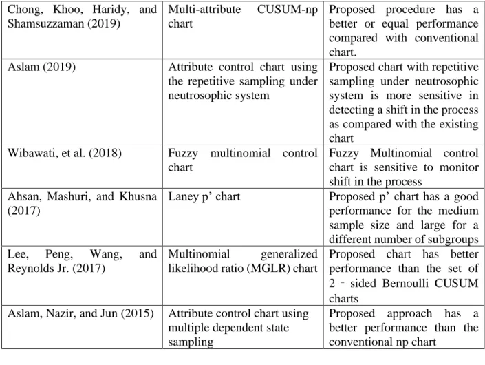
Chong, Khoo, Haridy, and Shamsuzzaman (2019)

Multi-attribute CUSUM-np chart

Proposed procedure has a better or equal performance compared with conventional chart.

Aslam (2019) Attribute control chart using the repetitive sampling under neutrosophic system

Proposed chart with repetitive sampling under neutrosophic system is more sensitive in detecting a shift in the process as compared with the existing chart

Wibawati, et al. (2018) Fuzzy multinomial control chart

Fuzzy Multinomial control chart is sensitive to monitor shift in the process

Ahsan, Mashuri, and Khusna (2017)

Laney p’ chart Proposed p’ chart has a good performance for the medium sample size and large for a different number of subgroups Lee, Peng, Wang, and

Reynolds Jr. (2017)

Multinomial generalized likelihood ratio (MGLR) chart

Proposed chart has better performance than the set of 2 ‐ sided Bernoulli CUSUM charts

Aslam, Nazir, and Jun (2015) Attribute control chart using multiple dependent state sampling

Proposed approach has a better performance than the conventional np chart

Table 3 The recent development in Mixed control chart

Ahsan et al., (2019b) PCA Mix chart for detecting outlier

Proposed chart has a great performance to detect more outlier with the higher percentage of outlier added compared to the conventional and other robust charts

Ahsan, et al., (2018) PCA Mix control chart Proposed chart presents good performance for an appropriate number of principal components used Wang, Su, Fang, and Zhang

(2018)

Multivariate sign chart Simulations show the superiority of proposed control chart in monitoring mixed type data

(28)

Furthermore, the recent development of the mixed control chart is presented in Table 3. For this area, it can be seen that there are a few works studied the mixed monitoring variable and attribute characteristics. Therefore, the more development for this area is needed. This research is trying to develop and assed the performance of the Mixed type chart, especially PCA Mix control chart, in order to bring a contribution for the monitoring process procedure.

3. Charting Procedures of PCA Mix Chart

This section discusses the procedures to form the multivariate control chart based on PCA Mix. Figure 1 illustrates the procedures in creating the multivariate control chart based on PCA Mix. In the procedure, there are three main steps. The first step is calculating the PCs using PCA Mix from the mixed characteristics. The second step is calculating the T² statistics from some principal components. Finally, estimate the control limit of the proposed chart using KDE. The detailed PCA Mix control chart procedure can be found in Ahsan et al. (2018).

PCA Mix Control Chart’s procedures

Step 1 Input the variable data X1 and the attribute data X2.

Step 2 Calculate the principal component scores (PCs) mix, denoted as

Y

^mix, using the PCA Mix method from X1 and X2.

Step 3 Take the first v components and calculate the

2 2 ,

1 ,

( )

,

l mix

i v v

i

v mix v

T y 

= 

=



− ^where is the ^v

eigenvalue respects to the v-th PCs.

Step 4 Calculate the empirical density of T_i²statistics,

2 2

2

1

ˆ ( )_h 1 ⁿ ⁱ

i

T T

f T k

nh = h

 − 

=  

 



^{, where}^h^{is the}

optimum bandwidth calculated using Botev, Grotowski, & Kroese (2010) algorithm.

Step 5 Calculate the distribution function T_i²statistics,

t2

2 2

0

( ) ˆ ( )

h h

F t =



f T dT ^.

1( )(1 ),

CL=F⁻ t − 

(29)

Figure 1 PCA Mix control chart procedures

4. Performance for Detecting Outlier

This section shows the performance of the proposed chart in detecting outlier mixed with the in-control data. In assessing its performance, the simulation studies with some scenarios are conducted. For the simulations, the variable characteristics are assumed to follow the Multivariate Normal Distribution X₁~N_p(0, I), while the attribute characteristics are generated to follow the Multinomial Distribution with three categories X₂ M( ,  ₁ ₂, ₃). Similar to the Ahsan et al.

(2019), the attribute characteristics are differentiated into three types such as the almost balanced proportion ( ₁, ₂ =0.3 and ₃ =0.4 ), imbalanced proportion ( ₁, ₂ =0.1 and ₃ =0.8 ), and extreme imbalanced proportion ( ₁, ₂ =0.05 and ₃=0.9).

For the detailed performance, the number of attribute characteristics is evaluated for 2, 3, and 5. On the other hand, the number of variable characteristics is 5. The outliers mixed with the clean data are set to 5, 10, 20, 30, 40, and 50 percent out of the total observations. There are three

(30)

misdetection with criteria of the lower the better. The detailed algorithm for this simulation studies can be found in Ahsan et al. (2019).

4.1 Two attribute characteristics

Table 4 shows the performance of the proposed chart in detecting outlier for two attribute characteristics with  ₁, ₂ =0.3 and ₃ =0.4. In general the proposed chart still has a stable performance for no more than 30 percent outlier added to the clean data. For this case, it can be seen that the misdetection occurs due to a large number of the in-control data declared as an outlier (high FP rate). The proposed chart performance in detecting outlier for two attribute characteristics with imbalanced proportion is reported in Table 5. Different from the previous case (two variable with balanced proportion), the misdetections are caused by the inability of the control chart to capture the actual outliers which can be seen from the high FN rate. Furthermore, Table 6 presents the performance of the proposed chart to detect outlier for the extreme imbalanced proportion ( ₁, ₂ =0.05 dan ₃=0.9). For this condition, it can be seen that the high value of the FN rate causes a low level of accuracy of the proposed chart. In general, for this case, using the number of component l=2 produces better results.

Table 4 Performance of the proposed chart in detecting outlier for two attribute characteristics with  ₁, ₂ =0.3 and ₃ =0.4

ε=5% ε=10%

Hit Rate FN Rate FP Rate Hit Rate FN Rate FP Rate p=5, l =2 0.96966 0.0000 0.0319 0.95122 0.0002 0.0542 p=5, l =3 0.97353 0.0000 0.0279 0.95445 0.0005 0.0506 p=5, l =4 0.96633 0.0000 0.0355 0.94993 0.0001 0.0556

ε=20% ε=30%

ε=40% ε=50%

(31)

Table 5 Performance of the proposed chart in detecting outlier for two attribute characteristics with  ₁, ₂ =0.1 and ₃=0.8

ε=5% ε=10%

ε=20% ε=30%

ε=40% ε=50%

Table 6 Performance of the proposed chart in detecting outlier for two attribute characteristics with  ₁, ₂ =0.05 and ₃ =0.9.

ε=5% ε=10%

ε=20% ε=30%

ε=40% ε=50%

(32)

4.2 Three attribute characteristics

The performance of the proposed chart in detection outlier in the case of three attribute characteristics with  ₁, ₂ =0.3 and ₃ =0, 4(balanced) is presented in Table 7. Similar to the two attribute characteristics case, the misdetection for this case happens due to the high false alarm produced represented by the high value of FP rate. Table 8 and 9 show the performance for three attribute characteristics with imbalanced and extreme imbalanced proportion, respectively. In this case, it can be seen that the misdetection for these two cases happens due to the actual outliers are failed to be detected represented by the high value of FN rate. From this case, it also can be seen that using smaller principal components produces better results. The performance degradation can be seen when the proposed chart monitors more than 30 percent outliers. Also, the more imbalanced proportion of the attribute characteristics the higher accuracy level produced.

Table 7 Performance of the proposed chart in detecting outlier for three attribute characteristics with  ₁, ₂ =0.3 and ₃ =0.4

ε=5% ε=10%

Hit Rate FN Rate FP Rate Hit Rate FN Rate FP Rate p=5, l =2 0.96961 0.0004 0.0320 0.95411 0.0001 0.0510 p=5, l =3 0.94098 0.0000 0.0621 0.92895 0.0003 0.0789 p=5, l =4 0.94272 0.0000 0.0603 0.91451 0.0000 0.0950

ε=20% ε=30%

ε=40% ε=50%

(33)

Table 8 Performance of the proposed chart in detecting outlier for three attribute characteristics with  ₁, ₂ =0.1 and ₃=0.8

ε=5% ε=10%

ε=20% ε=30%

ε=40% ε=50%

Table 9 Performance of the proposed chart in detecting outlier for three attribute characteristics with  ₁, ₂ =0.05 and ₃ =0.9.

ε=5% ε=10%

ε=20% ε=30%

ε=40% ε=50%

(34)

4.4 Five attribute characteristics

Table 10 shows the outlier monitoring results for five attribute data with

1, 2 0.3 and 3 0.4.

  =  = According to the simulation results, it can be concluded that, in this case, the misdetection occurs due to a large number of the in-control data declared as an outlier (see FP rate). The performances of the proposed chart for  ₁, ₂=0.1 and ₃=0.8 as well as

1, 2 0.05 and 3 0.9

  =  = are reported in Table 11 and 12, respectively. Similar to the two previous cases, the failure to detect the actual outliers leads to reduced accuracy given by the proposed chart.

In general, the usage of the smaller principal component leads to higher accuracy. This chart still at its peak performance for less than 40 percent outlier mixed. Moreover, the more imbalanced proportion of the attribute characteristics monitored by the proposed chart the higher Hit rate or accuracy produced.

Table 10 Performance of the proposed chart in detecting outlier for five attribute characteristics with  ₁, ₂ =0.3 and ₃ =0.4

ε=5% ε=10%

Hit Rate FN Rate FP Rate Hit Rate FN Rate FP Rate p=5, l=2 0.99097 0.0010 0.0095 0.98861 0.0035 0.0123 p=5, l =3 0.98939 0.0024 0.0110 0.98264 0.0040 0.0188 p=5, l =4 0.98968 0.0016 0.0108 0.98590 0.0051 0.0151

ε=20% ε=30%

ε=40% ε=50%