Arena Basics
The working simulation tool for the models in this book is Arena. Arena is a simulation environment consisting of module templates, built aroundSIMANlanguage constructs and other facilities, and augmented by a visual front end. This chapter provides an overview of Arena basics at an introductory level. For more detail, refer to Kelton et al. (2004). Because it may be hard to distinguish between Arena terms and generic terms, we shall always italicize any technical Arena terms throughout the book. Furthermore, we will adopt the notational convention that all characters in SIMAN constructs are always uppercase, while only the first character in Arena constructs is capitalized, and both are italicized.
SIMAN consists of two classes of objects: blocksand elements. More specifically, blocks are basic logic constructs that represent operations; for example, aSEIZEblock models the seizing of a service facility by a transaction (referred to in Arena as“entity”), while a RELEASEblock releases the facility for use by other transactions. Elements are objects that represent facilities, such as RESOURCES and QUEUES, or other components, such asDSTATSandTALLIES, used for statistics collection.
Arena's fundamental modeling components, called modules, are selected from template panels, such asBasic Process, Advanced Process, and Advanced Transfer,1 and placed on a canvas in the course of model construction. A module is a high-level construct, composed of SIMAN blocks and/or elements. For example, aProcessmodule models the processing of an entity, and internally consists of such blocks asASSIGN, QUEUE,SEIZE,DELAY, and RELEASE. Arena also supports other modules, such as Statistic,Variable, and Outputamong many others. Frequently used Arena constructs (built-in variables and modules) are succinctly described in Appendix A.
Arena implements a programming paradigm that combines visual and textual programming. A typical Arena session involves the following activities:
1. Selecting module/block icons from a template panel, and placing them on a graphical model canvas (by drag and drop).
1
Earlier versions of Arena have other panels, such asBlocks,Elements,Common, andSupport. Later versions of Arena preserve these legacy panels in a template panel directory calledOldArena Templates, and allow users to use them as necessary.
Simulation Modeling and Analysis with Arena
2. Connecting modules graphically to indicate physical flow paths of transactions and/or logical flow paths of control.
3. Parameterization of modules or elements using a text editor.
4. Writing code fragments in modules using a text editor. Arena code is case-insensitive; that is, upper and lower case letters are interchangeable.
Arena has a graphical user interface (GUI) built around the SIMAN language. In fact, simulation models can be built using SIMAN constructs from the Blocks and Elementstemplate panels alone, since Arena modules are just subprograms written in SIMAN. Still, Arena is far more convenient than SIMAN, because it provides many handy features, such as high-level modules for model building, statistics definition and collection, animation of simulation runs (histories), and output report generation. Model building tends to be particularly intuitive, since many modules represent actual sub-systems in the conceptual model or the real-life system under study. Complex models usually require both Arena modules and SIMAN blocks.
All in all, Arena provides a module-oriented simulation environment to model practically any scenario involving the flow of transactions through a set of processes. Furthermore, while the modeler constructs a model interactively in both graphical and textual modes, Arena is busy in the background transcribing the whole model into SIMAN. Since Arena generates correct SIMAN code and checks the model for syntactic errors (graphical and textual), a large amount of initial debugging takes place automatically.
5.1
ARENA HOME SCREEN
An Arena home screen is shown in Figure 5.1.
The reader is encouraged to browse the Arena home screen, and examine the objects to be mentioned in the sequel.
Project Bar
Animate Transfer Toolbar Title Bar Integration Toolbar Run Interaction Toolbar
Model Window Canvas
The Arena home screen has aTitlebar with the model name at its top. Below theTitle bar is the ArenaMenubar, which consists of a set of general menus and Arena-specific menus. Below theMenubar is a set of Arena toolbars that can be displayed and hidden by clicking the right mouse button on the background area of a specific toolbar. These toolbars consist of buttons that support model building and running; note that some toolbar buttons conveniently duplicate the functionality of certain menu options in theMenubar.
The bulk of the home screen is allocated to a model window canvas consisting of a flowchartview andspreadsheet view. The user spawns modules and other objects, drags them into the flowchart view canvas, and progressively builds a model from component modules selected from theProjectbar (on the left) with the aid of support functions. Selecting a module in the flowchart view pops up a spreadsheet view (below the flowchart view) that summarizes all module information and permits editing of the associated data.
In addition to theProjectbar, the user can also pop up (or hide) two additional bars below the model window canvas. TheDebugbar permits the user to track the evolution of simulation runs, while theStatusbar (below it) displays instructions and feedback messages concerning user actions.
The Menu bar and the set of key Arena toolbars are described next. Consult the online help for complete descriptions of all Arena bars (menu bars, toolbars, and so on).
5
.
1
.
1
M
ENUB
ARThe Arena Menu bar consists of a number of general menus—File, Edit, View, Window, andHelp—which support quite generic functionality. It also has the following set of Arena-specific menus:
TheToolsmenu provides access to simulation related tools and Arena parameters.
TheArrangemenu supports flowcharting and drawing operations. TheObjectmenu supports module connections and submodel creation.
TheRunmenu provides simulation run control. ItsSetup
. . .option opens a form that
permits the user to enter information, such as project parameters (name, analyst, date, etc.), as well as replication parameters (length, warm-up period, etc.). It also has options that provide VCR-type functionality to run simulation replications and run control options to monitor entity motion, variable assignments, and so on.
5
.
1
.
2
P
ROJECTB
ARTheBasic Processtemplate panel consists of a set of basic modules, such asCreate,
Dispose,Process,Decide,Batch,Separate,Assign, andRecord.
TheAdvanced Process template panel provides additional basic modules as well as
more advanced ones, such asPickup,Dropoff, andMatch.
TheAdvanced Transfertemplate panel consists of modules that support entity transfers
in the model. These may be ordinary transfers or transfers using material-handling equipment.
TheReportstemplate panel supports report generation related to various components in
a model, such as entities, resources, queues, and so on.
TheBlockstemplate panel contains the entire set of SIMAN blocks.
The Elements template panel contains elements needed to declare model resources,
queues, variables, attributes, and some statistics collection.
In addition to the Arena template panels above, the following Arena template panels from earlier versions are also supported:
TheCommontemplate panel contains Arena modules such asArrive,Server,Depart,
Inspect, and so on, as well as element modules such asStats,Variables,Expressions, andSimulate.
TheSupporttemplate panel contains a subset of frequently used SIMAN blocks.
The models we present in this book will mostly utilize modules from template panels of Arena 10.0 and later versions.
5
.
1
.
3
S
TANDARDT
OOLBARThe Arena Standard toolbar contains buttons that support model building. An important button in this bar is theConnectbutton, which supports visual programming. This button is used to connect Arena modules as well as SIMAN blocks, and the resulting diagram describes the flow of logical control. TheTime Patterns Editorfeature consists of three buttons that allow the modeler to schedule the availability of resources and their service rate. TheStandardtoolbar also provides VCR-style buttons to run an Arena model in interrupt mode to trace its evolution. More details on this VCR-like functionality are discussed in Section 6.3.1.
5
.
1
.
4
D
RAWANDV
IEWB
ARSTheDrawtoolbar supports static drawing and coloring of Arena models. In a similar vein, theViewtoolbar (not shown in Figure 5.1) assists the user in viewing a model. Its buttons includeZoom In,Zoom Out,View All, andView Previous. These functions make it convenient to view large models at various levels of detail.
5
.
1
.
5
A
NIMATE ANDA
NIMATET
RANSFERB
ARSAnimate Transfertoolbar is used to animate entity transfer activities, including materials handling (see Section 13.2 for more details).
5
.
1
.
6
R
UNI
NTERACTIONB
ARThe Run Interaction toolbar supports run control functions to monitor simulation runs, such as access to SIMAN code and model debugging facilities. It also supports model visualization, such as theAnimate Connectors button that switches on and off entity traffic animation over module connections. Because of this toolbar's fundamental role in model testing, it will be revisited in Chapter 6.
5
.
1
.
7
I
NTEGRATIONB
ARTheIntegrationtoolbar supports data transfer (import and export) to other applica-tions. It also permits Visual Basic programming and design. A primer on Visual Basic for Arena may be found in Appendix B.
5
.
1
.
8
D
EBUGB
ARTheDebugtoolbar supports debugging of Arena models by monitoring and controlling the execution of a simulation run. It consists of two subwindows. The left subwindow can be used in command mode to set breakpoints, assign variable values, observe watched variables, and trace entity flows among modules. The right subwindow has tabs for viewing future SIMAN events in the model, displaying attributes of the current active entity, and watching user-defined Arena expressions. For more information, see Chapter 6.
5.2
EXAMPLE: A SIMPLE WORKSTATION
We now proceed to illustrate the basic features of Arena through a simple example. Consider a single workstation consisting of a machine with an infinite buffer in front of it. Jobs arrive randomly and wait in the buffer while the machine is busy. Eventually they are processed by the machine and leave the system. Job interarrival times are exponentially distributed with a mean of 30 minutes, while job processing times are exponentially distributed with a mean of 24 minutes. This system is known in queueing theory as theM/M/1queue (Kleinrock 1975).
The steady-state behavior of this system has been well studied, and analytical formulas have been derived for its main performance measures, such as distribution of the number of jobs in the system and average waiting time in the buffer (seeibid.) This example will compare the simulation statistics to their theoretical counterparts to gauge the accuracy of simulation results. Specifically, we shall estimate by an Arena simulation the average job delay in the buffer, the average number of jobs in the buffer, and machine utilization.
Simulating the above workstation calls for the following actions:
2. If the machine is busy processing another job, then the arriving job is queued in the buffer.
3. When a job advances to the head of the buffer, it seizes the machine for processing once it becomes available, and holds it for a time period sampled from the prescribed processing-time distribution.
4. On process completion, the job departs the machine and is removed from the system (but not before its contribution to the statistics of the requisite perform-ance measures are computed).
A simple approach to modeling the workstation under study is depicted in Figure 5.2.
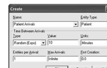
In this model, jobs (Arena entities) are created by theCreatemoduleCreate 1. Jobs then proceed to be processed in theProcessmoduleProcess 1, after which they enter theDisposemodule,Dispose 1, for removal from the model. The graphic shaped like an elongated T (called aT-bar) above the moduleProcess 1represents space for waiting jobs (here, the workstation's buffer). The interarrival specification of theCreatemodule is shown in the dialog box of Figure 5.3.
The dialog box contains information on job interarrival time(Time Between Arrivals section), batch size (Entities per Arrivalfield), maximal number of job arrivals (Max Arrivals field), time of first job creation (First Creation field), and so on. The Type pull-down menu in theTime Between Arrivalssection offers the following options:
Random(exponential interarrival times with mean given in theValuefield)
Schedule(allows the user to create arrival schedules using theSchedulemodule from
theBasic Processtemplate panel)
Figure 5.3 Dialog box for aCreatemodule.
Constant(specifies fixed interarrival times)
Expression (any type of interarrival time pattern specified by an Arena expression,
including Arena distributions)
The job processing mechanism (including priorities) is specified in the Process module, whose dialog box is shown in Figure 5.4.
TheActionfield option, selected from the pull-down menu, isSeize Delay Release, which stands for a sequence ofSEIZE,DELAY, andRELEASESIMAN blocks.SEIZE andRELEASEblocks are used to model contention for a resource possessing a capacity (e.g., machines). When resource capacity is exhausted, the entities contending for the resource must wait until the resource is released. Thus theSEIZEblock operates like a gate between entities and a resource. When the requisite quantity of resource becomes available, the gate opens and lets an entity seize the resource; otherwise, the gate bars the entity from seizing the resource until the requisite quantity becomes available. Note that the resource quantity seized should be an integer; otherwise Arena truncates it.
The processing (holding) time of a resource (Machine in our case) by an entity is specified via theDELAYblock within theProcessmodule. For instance, the dialog box of Figure 5.4 specifies that one unit of resource Machine be seized and held for an exponentially distributed time with a mean of 24 minutes. If multiple resources need to be seized simultaneously, all requisite resources are listed, and the holding time clock is started only afterallrequisite resources listed become available. When at least one of the listed resources is not available, arriving entities wait in a FIFO (First In First Out) queue, ordered further by priorities (specified in thePriority field of the dialog box). This discipline is called FIFO within priority classes, because higher-priority entities precede lower-priority ones, but arrivals within a given priority class are ordered FIFO.
TheAddbutton in aProcessmodule (see Figure 5.4) is used to specify resources and the resource quantities to be seized by an incoming entity. To this end, theAddbutton pops up aResourcesdialog box as shown in Figure 5.5.
Note, however, that the capacity of resources introduced in aResourcesdialog box is specified elsewhere, namely, in theResourcemodule spreadsheet (Figure 5.6).
This spreadsheet is accessible in theBasic Processtemplate of theProjectbar, and is used to specify all resource capacities of an Arena model. The default capacity of resources is 1. More details on the Resource module spreadsheet are deferred to examples in the sequel.
TheDisposemodule implements an entity“sunset”mechanism, by simply discard-ing entities that enter it. As such, theDisposemodule serves as a system“sink,”thereby counteracting theCreatemodule, which serves as a system“source.”Note carefully that in the absence of properly placedDisposemodules, the number of entities created in the course of a simulation run can grow without bound, eventually exhausting available computer memory (or a prescribed limit) and terminating the run (very likely crashing the simulation program). ADisposemodule is not necessary, however, when a fixed or bounded number of entities are created and circulate in the system indefinitely.
Whenever an Arena model is saved, the model is placed in a file with a .doe extension (e.g.,mymodel.doe). Furthermore, whenever a model, such asmymodel.doe, is checked using theCheck Modeloption in theRunmenu or any run option in it, Arena automatically creates a number of files for internal use, includingmymodel.p(program file), mymodel.mdb (Access database file), mymodel.err (errors file), mymodel.opw (model components file), andmymodel.out (SIMAN output report file). As these are internal Arena files, the modeler should not attempt to modify them.
Figure 5.6 Resourcemodule spreadsheet for specifying resource capacities.
Run control functionality is provided by theRunpull-down menu (see Figure 5.1). Selecting the Setup. . . option opens the Run Setup dialog box, which consists of
multiple tabs, each with its own dialog box. In particular, theReplication Parameters tab permits the specification of the number of replications, replication length, and the warm-up period. (A warm-up period is a simulation of an initial interval, designed to “warm up”the system to a more representative state; this will be discussed in greater detail in Chapter 9 when we discuss output analysis.) In this example, the model will be simulated for 10,000 hours, with all other fields in theRun Setupdialog box retaining their default values.
The end result of a simulation run is a set of requisite statistics, such as mean waiting times, buffer size probabilities, and so on. These will be referred to asrun results. Arena provides a considerable number of default statistics in a report, automatically generated at the end of a simulation run. Additional statistics can be obtained by adding statistics-collection modules to the model, such asRecord (Basic Processtemplate panel) and Statistic (Advanced Process template panel). However, when using SIMAN (the Support template panel in the Old Arena Templates folder), the user has to include additional blocks and elements in the model in order to affect statistics collection. The simpler statistics-collection facilities in Arena are one of the advantages of Arena over SIMAN. Subsequent chapters will provide additional information on statistics collection.
The run results of a single replication of the workstation model from Figure 5.2 are displayed in Figures 5.7 and 5.8.
Figure 5.7 displays the Resources section, which includes resource utilization. The last three columns correspond to the half-width of the confidence interval (see Section 3.10), minimum observation, and maximum observation, respectively, of the corresponding statistics. The(insufficient)notation indicates that the number of obser-vations is insufficient for adequate statistical confidence. Observe that theNumber Busy item refers to the number of busy units of a resource, while theNumber Scheduleditem refers to resource capacity. TheInstantaneous Utilizationitem pertains to utilization per
resource unit, namely,Number Busydivided by theNumber Scheduled. We point out that in the long run, individual resource utilizations approach this number.
Figure 5.8 displays theQueuessection, which consists of customer-oriented statistics (customer averages), such as mean waiting times in queues, as well as queue-oriented statistics, such as time averages of queue sizes (occupancies). Additional sections in an output report includeFrequencies(probability estimates) and User Specified(any customized statistics). For more details on Arena statistics collection and output reporting, see Sections 5.4 and 5.5.
An examination of the run results (replication statistics) displayed in Figures 5.7 and 5.8 reveals that the machine utilization is about 81%. The average waiting time in the machine buffer is about 107 minutes, with a 95% confidence interval of 107.0916.42523 minutes, and a maximum of 807.06 minutes. The average number
of jobs in the buffer is 3.57 jobs, with the maximal buffer length observed being 35 jobs. Figure 5.7 can be used for preliminary verification of the workstation model. For example, we can use the classical formula r¼l=m (Kleinrock 1975) of machine utilization to verify that the observed server utilization, r, is indeed the ratio of the job arrival rate (l¼1=30) and the machine-processing rate (m¼1=24). Indeed, this ratio is 0.8, which is in close agreement with the run result, 0.8097. Note that this relation holds only approximately, due to the inherent variation in sampling simulation statistics. Other verification methods will be covered in some detail in Chapter 8.
5.3
ARENA DATA STORAGE OBJECTS
An important part of the model building process is assignment and storage of data supplied by the user (input parameters) or generated by the model during a simulation run (output observations). To this end, Arena provides three types of data storage objects:variables,expressions, andattributes. Variables and expressions can be intro-duced and initialized via theVariable andExpressionspreadsheet modules, accessible from theBasic Processtemplate andAdvanced Processtemplate, respectively, in the Projectbar.
5
.
3
.
1
V
ARIABLESVariablesare user-definedglobaldata storage objects used to store and modify state information at run initialization or in the course of a run. Such (global) variables are visible everywhere in the model; namely, they can be accessed, examined, and modified from every component of the model. In an Arena program, variables are typically examined in Decide modules and modified in Assign modules. Unlike user-defined variables, certain predefined Arena (system) variables are read-only (i.e., they may only be examined to decide on a course of action or to collect statistics), and cannot be assigned a new value by the user; the system is solely responsible for changing these values. For instance, the variableNQ(Machine_Q) stores the current value of the number of entities in the queue calledMachine_Q. Similarly, the variableNR(Machine) stores the number of busy units of the resource calledMachine. Other important Arena variables areTNOW, which stores the simulation run's current time (simulation clock), andTFIN, which stores the simulation completion time. A list of all Arena variables may be found in theArena Variables Guideor in the ArenaHelpfacility (see Section 6.6). Recall that a selected partial list appears in Appendix A.
5
.
3
.
2
E
XPRESSIONSExpressionscan be viewed as specializedvariablesthat store the value of an associ-ated formula (expression). They are used as convenient shorthand to compute mathemat-ical expressions that may recur in multiple parts of the model. Whenever an expression name is encountered in the model, it is promptly evaluated at that point in simulation time, and the computed value is substituted for the expression name. Variables of any kind (user defined or system defined) as well as attributes may be used in expressions.
5
.
3
.
3
A
TTRIBUTESAttributesare data storage objects associated with entities. Unlike variables, which are global, attributes are local to entities in the sense that each instance of an entity has its own copy of attributes. For example, a customer's arrival time can be stored in a customer attribute to allow the computation of individual waiting times. When arrivals consist of multiple types of customer, the type of an arrival can also be stored in a customer entity’s attribute to allow separate statistics collection for each customer type.
5.4
ARENA OUTPUT STATISTICS COLLECTION
Arena provides two basic mechanisms for collecting simulation output statistics: one via theStatistic module, and the other via theRecordmodule. Time average statistics are collected in Arena via theStatisticmodule, while customer-average statistics must be collected via aRecord module, and (optionally) specified in theStatisticmodule. Arena statistics collection mechanisms are described next in some detail.
5
.
4
.
1
S
TATISTICSC
OLLECTION VIA THES
TATISTICM
ODULEDetailed statistics collection in Arena is typically specified in the Statisticmodule located in theAdvanced Processtemplate panel. Selecting theStatisticmodule opens a dialog box. The modeler can then define statistics as rows of information in the spreadsheet view that lists all user-defined statistics. For each statistic, the modeler specifies a name in theNamecolumn, and selects the type of statistic from a drop-down list in theTypecolumn. The options are as follows:
Time-Persistent statistics are simply time average statistics in Arena terminology. Typical Time-Persistent statistics are average queue lengths, server utilization, and various probabilities. Any user-defined probability or time average of an expression can be estimated using this option.
Tallystatistics are customer averages, and have to be specified in aRecordmodule (see Section 5.4.2) in order to initiate statistics collection. However, it is advisable to include the definition in the Statisticmodule as well, so that the entire set of statistics can be viewed in the same spreadsheet for modeling convenience. Counterstatistics are used to keep track of counts, and like theTallyoption, have to
be specified in aRecordmodule (see Section 5.4.2) in order to initiate statistics collection.
Outputstatistics are obtained by evaluating an expression at the end of a simulation run. Expressions may involve Arena variables such asDAVG(S)(time average of theTime-PersistentstatisticS),TAVG(S) (the average of Tally statisticS),TFIN (simulation completion time),NR(),NQ(), or any variable from theArena Vari-ables Guide.
Frequency statistics are used to produce frequency distributions of (random) expres-sions, such as Arena variables or resource states. This mechanism allows users to estimate steady-state probabilities of events, such as queue occupancy or resource states.
Note that all statistics defined in theStatistic module are reported automatically in theUser Specified section of the Arena output report (see Section 5.5). Furthermore, Queue and Resource Time-Persistent statistics will be automatically computed and need not be defined in theStatisticmodule.
5
.
4
.
2
S
TATISTICSC
OLLECTION VIA THER
ECORDM
ODULEThese options are as follows:
1. The Count option maintains a count with a prescribed increment (positive or negative). The increment is quite general: it may be defined as any expression or function and may assume any real value. The corresponding counter is incremented whenever an entity enters theRecordmodule.
2. The Entity Statistics option provides information on entities, such as time and costing/duration information.
3. TheTime Interval option tallies the difference between the current time and the time stored in a prescribed attribute of the entering entity.
4. TheTime Betweenoption tallies the time interval between consecutive entries of entities in theRecordmodule. These intervals correspond to interdeparture times from the module, and the reciprocal of the mean interdeparture times is the module’sthroughput.
5. Finally, the Expression option tallies an expression whose value is recomputed whenever an entity enters theRecordmodule.
Note that except for theEntity Statisticsoption, all the options above are implemented in SIMAN viaCOUNTorTALLYblocks.
5.5
ARENA SIMULATION AND OUTPUT REPORTS
An Arena model run can be initiated and managed in two ways:
Via the VCR-like buttons on the ArenaStandardtoolbar Via corresponding options in theRunpull-down menu bar
Refer to Section 6.3 for more details.
Standard Arena output reports provide summaries of simulation run statistics, as requested by the modeler implicitly or explicitly. Accordingly, Arena output reports fall into two categories:
Automatic reports. A number of Arena constructs, such as entities, queues, and resources, will automatically generate reports of summary statistics at the end of
a simulation run. Those statistics are implicitly specified by the modeler simply by dragging and dropping those modules into an Arena model, and no further action is required of the user.
User-specified reports. Reports on additional statistics can be obtained by explicitly specifying statistics collection via the Statistic module (Advanced Process template panel) and the Record module (Basic Process template panel). Recall that the Statistic module is specified in a spreadsheet view, while the Record module must be placed in the appropriate location in the model.
To request a formatted report, the user opens theReportspanel in theProjectbar to display a list of report options that correspond to various types of statistics as follows:
Entitiesreports automatically provide various entity counts.
Frequenciesreports provide time averages of expressions (including probabilities as
a special case). The expression must be specified in a Statistic module with the Frequencyoption selected.
Processes reports provide statistics associated with each Process module. These
include incoming and outgoing entity counts, average service times, and average delays. Time-oriented statistics (e.g., delays) include the average, half-width of 95% confidence intervals, and minimal and maximal observed values. The half-width value is not displayed if the observations are correlated or if there are insufficient data (in which case Arena prints(insufficient)in the corresponding field).
Queuesreports provide statistics for each queue in the model, such as average queue
delay and average queue size. Additional statistics include the half-width of the 95% confidence interval, and minimal and maximal observed values.
Resourcesreports provide statistics for each resource in the model, such as utilization,
average number of busy resource units, and number of times seized.
User Specified reports are generated in response to explicit modeler requests for
statistics collection in theStatisticmodule orRecordmodules (see Section 5.4). These include anyTime-Persistent,Tally,Count,Frequency, andOutputstatistics.
Clicking on a report option in theReportstemplate panel of theProjectbar prompts Arena to format the corresponding report and display it in a window. The top of that window contains VCR-like navigation buttons allowing the user to navigate report pages. Any number of options may be selected (sequentially), and the resultant report generated by Arena will consist of corresponding report sections. TheToggle Group Treebutton at the top of the report window pops up aPreviewpanel to aid in navigating report sections.
5.6
EXAMPLE: TWO PROCESSES IN SERIES
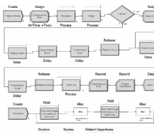
is a painting operation that takes 3 hours per job. We are interested in simulating the system for 100,000 hours to obtain process utilizations, average number of reworks per job, average job waiting times, and average job flow times (elapsed times experienced by job entities). Figure 5.10 depicts the corresponding Arena model and a snapshot of its state.
In this Arena model, entities represent jobs that are created by the Createmodule Job Arrivals, and enter the Assign module Arrival Time, where their arrival time is assigned to an attribute calledArrTime. Job entities then proceed to theProcessmodule Assembly, where they undergo assembly. Next, assembled job entities go through inspection in theDecidemoduleQuality Check, and those needing rework are routed to theAssignmoduleNumber of Reworksto record the number of reworks per job, and then back to moduleAssembly. Job entities that pass inspection proceed to be painted in theProcessmodulePainting, which completes the manufacturing operation. Completed job entities go through Record modules Flow Time and Reworks per Job to collect statistics of interest. Finally, job entities enter theDisposemoduleCompleted, where they are removed from the model.
The numbers at bottom right of the module icons display the number of entities that departed from the module. The icons above the moduleAssemblyrepresent jobs waiting in theAssemblyqueue, calledAssembly.Queue. TheVariablewindow at bottom left of the figure displays the number of the aforementioned jobs. Job icons and data displayed on the module aredynamic, that is, they change as the simulation run unfolds in time. For example, this snapshot indicates that at the time it was taken, 28 jobs were created, 20 jobs were completed, 7 jobs were waiting to be assembled, and 1 job was being assembled.
We next proceed to explain the modules used in the model in more detail (note that the default module names have been replaced here by more expressive names relevant to the problem at hand).
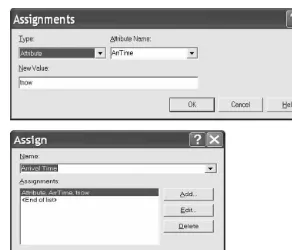
The arrival time assignment is carried out in theAssignmoduleArrival Time, whose dialog boxes are shown in Figure 5.11.
Note that the bottom dialog box appears first on the screen, while clicking on an item in itsAssignmentsfield pops up the top dialog box for entering a value for the corresponding variable or attribute.
The moduleAssemblyin Figure 5.10 is, in fact, aProcess module that models the assembly operation with the appropriate job assembly time specification. Recall that the T-bar above the Process icon represents an animated Queue object for holding entities waiting for an opportune condition (e.g., to seize a resource). Note that the T-bar is displayed in aProcessmodule only if the module contains aSeizeoption. The dialog box of the moduleAssemblyin Figure 5.10 is displayed in Figure 5.12.
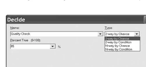
ADecidemodule, calledQuality Check, follows the assembly operation, represent-ing a quality control check. The Decide dialog box is shown in Figure 5.13. This module executes entity transfers, which may be probabilistic or based on the truth or falsity of some logical condition. Our example assumes that transfer times between processes are negligible, and therefore instantaneous. Here, we have a two-way probabilistic branchingthat splits the incoming stream of job entities into two outgoing streams:
With probability 0.85, an incoming job is deemed“good”(passed inspection), and is forwarded to theProcessmodule, calledPainting.
With probability 0.15 an incoming job is deemed “bad” (failed inspection), and is routed back to theProcessmodule, calledAssembly, for rework.
For convenience, the Type field provides separate options for simple two-way branching, which is the most common, as well as general n-way branching, which is more complex. In n-way branching, this module has multiple exits, exactly one
of which is designated theelsebranch and serves for default exits of entities from the module. More specifically, in probabilistic branching, a branch is taken with its associated probability, and theelse branch automatically complements the exit prob-abilities, ensuring that they sum to 1. Inconditional branching, the entity exits at the first branch whose condition evaluates to true, and if all conditions are false, the entity exits at theelsebranch.
Job entities that fail inspection enter theAssignmodule, calledNo of Reworks, where the job attribute, calledTotal Reworks, is incremented by the expressionTotal Reworks
þ1. The dialog box for this module is shown in Figure 5.14.
Job entities departing from the Painting module enter two Recordmodules called Flow TimeandReworks per Job, to record their flow times and total number of reworks per job, respectively. In our example, the flow time is the difference between the job
Figure 5.13 Dialog box of theDecidemoduleQuality Checkwith a two-way probabilistic branching.
departure time from thePaintingmodule and the job’s arrival time at moduleAssembly. Note that the job flow time includes any delays in queues as well as processing times. The average flow time is a customer average (Time Interval statistic), computed internally by a TALLY block, which can be verified by accessing the corresponding .modfile. The dialog box of theRecordmodule is shown in Figure 5.15.
In the next Record module, the expression consisting of the job entity’s attribute Total Reworksis tallied in theRecordmodule calledReworks per Job, as shown in the dialog box of Figure 5.16.
Figure 5.14 Dialog box of theAssignmoduleNo of Reworks.
Figure 5.15 Dialog box of aRecordmodule tallying job flow times.
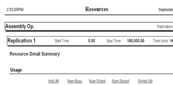
Finally, job entities proceed to be disposed of in the Dispose module, called Completed. A single replication of the model was run for 100,000 hours, and the results are displayed in Figures 5.17, 5.18, and 5.19.
Figure 5.17 Resource statistics for the manufacturing model (two processes in series).
Figure 5.18 Queue statistics for the manufacturing model (two processes in series).
Figure 5.17 shows that the utilization estimates of the Assemblerresource at the Assemblymodule and thePainterresource at thePaintingmodule are 0.94 and 0.59, respectively. These estimates in Figure 5.17 correspond to a heavy traffic regime in the former and a medium traffic regime in the latter. These result in long average buffer delays and large average buffer occupancy in the assembly process, and in short average buffer delays and low average buffer occupancy in the painting process as shown in Figure 5.18. Finally, the Tally section of the User Specified output in Figure 5.19 displays not only averages, but also the corresponding 95% confidence interval half-widths, as well as the minimal and maximal observations for the number of reworks and flow time per job. Note that some jobs underwent as many as four reworks, while the average number of reworks is just 0.18, indicating a low level of reworks. The average flow time (49.5252 hours) is moderately longer than the sum of the average delays in theAssembly and Painting queues (35.42 hours) and the sum of average processing times there (7 hours), due to additional rework performed at moduleAssembly.
5.7
EXAMPLE: A HOSPITAL EMERGENCY ROOM
This section presents a more detailed model—in this case, of an emergency room in a small hospital—to further illustrate the power of simulation modeling.
5
.
7
.
1
P
ROBLEMS
TATEMENTThe emergency room of a small hospital operates around the clock. It is staffed by three receptionists at the reception office, and two doctors on the premises, assisted by two nurses. However, one additional doctor is on call at all times; this doctor is summoned when the patient workload up-crosses some threshold, and is dismissed when the number of patients to be examined goes down to zero, possibly to be summoned again later. Figure 5.20 depicts a diagram of patient sojourn in the emergency room system, from arrival to discharge.
Patients arrive at the emergency room according to a Poisson process with mean interarrival time of 10 minutes. An incoming patient is first checked into the emergency room by a receptionist at the reception office. Check-in time is uniform between 6 and
Treatment
12 minutes. Since critically ill patients get treatment priority over noncritical ones, each patient first undergoestriagein the sense that a doctor determines the criticality level of the incoming patient in FIFO order. The triage time distribution is triangular with a minimum of 3 minutes, a maximum of 15 minutes, and a most likely value of 5 minutes. It has been observed that 40% of incoming patients arrive in critical condition, and such patients proceed directly to an adjacent treatment room, where they wait FIFO to be treated by a doctor. The treatment time of critical patients is uniform between 20 and 30 minutes. In contrast, patients deemed noncritical first wait to be called by a nurse who walks them to a treatment room some distance away. The time spent to reach the treatment room is uniform between 1 and 3 minutes and the treatment time by a nurse is uniform between 3 and 10 minutes. Once treated by a nurse, a noncritical patient waits FIFO for a doctor to approve the treatment, which takes a uniform time between 5 to 10 minutes. Recall that the queueing discipline of all patients awaiting doctor treatment isFIFO within their priority classes, that is, all patients wait FIFO for an available doctor, but critical patients are given priority over noncritical ones. Following treatment by a doctor, all patients are checked out FIFO at the reception office, which takes a uniform time between 10 and 20 minutes, following which the patients leave the emergency room.
The performance metrics of interest in this problem are as follows:
Utilization of the emergency room staff by type (doctors, nurses, and receptionists)
Distribution of the number of doctors present in the emergency room
Average waiting time of incoming patients for triage
Average patient sojourn time in the emergency room
Average daily throughput (patients treated per day) of the emergency room
To estimate the requisite statistics, the hospital emergency room was simulated for a period of 1 year.
5
.
7
.
2
A
RENAM
ODELHaving studied the problem statement, we now proceed to construct an Arena model of the system under study. Figure 5.21 depicts an Arena model of the emergency room system, where modules are labeled with their type to facilitate understanding.
The model is composed of two segments:
Emergency room segment. This logic (top segment of Figure 5.21) keeps track of
model entities (patients in our case), whose specification can be viewed and edited in the spreadsheet view of the Entity module from the Basic Process template panel. In this part of the model logic, a patient is generated and then moves through the emergency room processing, from admission to treatment to discharge.
On-call doctor segment. This logic (bottom segment of Figure 5.21) controls the
periodic summoning and dismissal of the extra doctor on call. This is achieved by a perpetually circulating single entity, calledadministratorin this model, which triggers the summoning and dismissal of the on-call doctor.
summary reports. We assume that the emergency room is initially empty and the on-call doctor is not present.
We next proceed to examine the Arena model logic of Figure 5.21 in some detail, including the role of common modules from theBasic ProcessandAdvanced Process template panels.
5
.
7
.
3
E
MERGENCYR
OOMS
EGMENTStarting at top left and moving to the right in the emergency room segment, the first module is the Create module, called Patient Arrivals, which generates incoming patient entities. Figure 5.22 displays the dialog box for this module, showing that patients arrive according to a Poisson process with exponential interarrival times of mean 10 minutes.
An incoming patient entity then enters the Assign module, calledRecord Arrival Time, where its arrival time is recorded in its ArrTime attribute. The value in this attribute will be carried by the patient entity throughout its sojourn in the emergency room system, and will be used later to compute its sojourn time (total time in the system).
The patient entity then promptly attempts to check into the emergency room by entering theProcessmodule, calledReception, whose dialog box is depicted in Figure 5.23.
At this juncture, the patient entity waits in line (if any) to seize a receptionist for a uniform check-in processing time between 6 and 12 minutes, after which the receptionist is released and becomes available to other patient entities. Note that theProcessmodule uses theSeize Delay Releaseoption in theActionfield, since receptionists are modeled as
Figure 5.22 Dialog box of theCreatemodulePatient Arrivals.
a resource, and the problem calls for computing expected waiting times and utilizations of the check-in operation. Once check-in is completed, the patient entity proceeds to the Processmodule, calledTriage, to undergo a triage checkout by a doctor. Figure 5.24 shows that a patient entity waits for a doctor to become available, and then undergoes a random triage time, drawn from the triangular distribution between 3 and 15 minutes, with a most likely time of 5 minutes.
After the triage delay is completed, the triage doctor is released and the patient entity proceeds to determine its level of criticality. To this end, it enters theDecidemodule, calledCritical?, whose dialog box is depicted in Figure 5.25.
In Figure 5.25, the2-Way by Chanceoption specifies a two-way random branching based on the result of a random experiment, and thePercent Truefield indicates that 40% of the time the result is true (so 60% of the time the result is false). Accordingly, the corresponding branches emanating from theDecidemoduleCritical?in Figure 5.21 are labeledtrueandfalse. Thus, a patient entity emerging from moduleCritical?takes either thetruebranch or thefalsebranch as follows:
Thetruebranch indicates that the patient is entity deemed critical. Such a patient entity will
proceed to be treated by a doctor. Recall that this applies to 40% of the patients.
Thefalsebranch indicates that the patient entity is deemed noncritical. Such a patient
entity will proceed to be treated by a nurse, and then will be inspected by a doctor, but at a lower priority than any critical patient entity.
The criticality level of patient entities is indicated in theirCriticalityattribute: a value of 1 codes for a critical patient, while a value of 0 codes for a noncritical patient. Accordingly, critical patient entities exiting module Critical? proceed to the Assign module, calledMark Critical, where theirCriticalityattribute is set to 1, as shown in the dialog box of Figure 5.26.
In contrast, noncritical patient entities are automatically marked as such, since the default value of theCriticalityattribute is 0 (recall that this is the Arena convention for all attributes). Such patient entities exiting module Critical? proceed to the Seize module, calledWaiting Room, whose dialog box is depicted in Figure 5.27.
In this module, noncritical patient entities wait FIFO in a queue, calledWaiting Room. Queue, for a nurse until one becomes available. Once a nurse is seized, the patient entity passes through two Delay modules in succession: module Move to Treatment Room models the uniformly distributed time between 1 and 3 minutes that it takes the nurse to walk a (noncritical) patient to a treatment room, while module Treatment by Nurse models the uniformly distributed time between 3 and 10 minutes that it takes the nurse to treat a patient. Figure 5.28 depicts the dialog boxes of these twoDelaymodules.
Having completed its treatment, the noncritical patient entity releases the nurse by entering the Release module, called Release Nurse, whose dialog box is shown in Figure 5.29.
At this point the paths of critical and noncritical patient entities converge, and all patient entities, both critical and noncritical, attempt to enter theSeizemodule, calledWait for Doctor. Note that an individualSeizemodule has the same functionality as theSeize
Figure 5.25 Dialog box of theDecidemoduleCritical?for determining patient criticality.
Figure 5.27 Dialog box of theSeizemoduleWaiting Room.
Figure 5.28 Dialog boxes of theDelaymodulesMove to Treatment Room(left) andTreatment by Nurse (right).
option in aProcessmodule, but with the added flexibility that the modeler can insert extra logic between the Seize and Delay functionalities (this is impossible in a Process module). The dialog box of theWait for Doctormodule is shown in Figure 5.30.
All patient entities wait in the queue, called Wait for Doctor.Queue to seize an available doctor, with critical patient entities receiving priority in treatment over noncritical ones. To this end, all patient entities queue upFIFO within priority classes, that is, all critical patient entities precede all noncritical ones, but each patient category is queued in the order of arrival. This is achieved by specifying the appropriate queueing discipline in theQueuemodule, whose spreadsheet view is shown in Figure 5.31.
Each row in the spreadsheet specifies a queue in the Arena model, while columns TypeandAttribute Namespecify jointly the queueing discipline. Observe that all rows, except row 4, specify the ordinary FIFO discipline, while row 4 implicitly specifies theFIFO within priority classesdiscipline. More specifically, patient entities in Wait for Doctor.Queue queue up FIFO, but their queueing priority is determined by their Criticalityattribute (the higher the value ofCriticality, the higher the priority).
Figure 5.31 Spreadsheet view of theQueuemodule specifying queueing disciplines.
Once a doctor becomes available, the patient entity at the head of the line seizes that doctor and proceeds to theDelay module, called Treatment by Doctor, whose dialog box is depicted in Figure 5.32.
Recall that the treatment duration of a patient depends on its level of criticality, namely, on itsCriticality attribute: for critical patients, the duration is uniform between 20 and 30 minutes, while for noncritical ones it is uniform between 5 and 10 minutes only. This dependence is captured in theDelay Timefield of Figure 5.32 by the expression
( Criticality¼¼1)
UNIF( 20,30)þ( Criticality¼¼0)
UNIF( 5,10):
Recall that(Criticality¼¼1)and (Criticality¼¼0) are logical expressions (predicates)
that return 1 or 0 according to logical value of the expression in parentheses, which evaluates to true or false, respectively. Thus, for critical patients the expression above reduces toUNIF(20,30), whereas for noncritical ones it reduces toUNIF(5,10), which are the requisite distributions.
Following treatment by a doctor, all patient entities proceed to theReleasemodule, calledRelease Doctor, where the doctor administering the treatment is released to other patients. Next, all patient entities are discharged from the emergency room. To this end, they enter theProcessmodule, calledCheck Out, whose dialog box is shown in Figure 5.33. The checkout procedure requires a patient to seize a receptionist for a uniform time between 10 and 20 minutes, before releasing that receptionist.
Finally, patient entities enter two statistics-collectingRecordmodules, calledPatient Sojourn TimeandPatient Departures, respectively, whose dialog boxes are depicted in Figure 5.34.
The first Recordmodule (left) tallies the total time that patient entities spend in the emergency room, from arrival to discharge (sojourn time)—a measure of patient satisfaction. This statistic is specified in theTypefield by theTime Intervaloption, and is computed as Tnow—ArrTime, namely, the difference between the current time and the patient's arrival
time as recorded in itsArrTimeattribute. The secondRecordmodule (right) simply counts the number of patient entities discharged from the emergency room—a measure of emergency room productivity. This statistic is specified in theTypefield by theCount option, and is computed by incrementing a counter variable, calledPatient Departures(see theCounter Namefield), whenever a patient entity enters this module. Note that the modeler can access the current value of any counter via the Arena variableNC(counter_name).
At long last, patient entities enter the Disposemodule, calledLeave Facility, after which they are removed from the model.
5
.
7
.
4
O
N-C
ALLD
OCTORS
EGMENTThe logic of this segment is controlled by a single circulating entity, dubbed administrator. The idea is to have the administrator modulate the number of doctors in the emergency room, depending on the number of patients in triage. Recall that emergency room doctors are a resource, so the administrator need only change this resource capacity as prevailing conditions change in the triage operation.
Figure 5.34 Dialog boxes of theRecordmodulesPatient Sojourn Time(left) andPatient Departures(right).
First, a single administrator entity is created at time 0, as shown in the dialog box of theCreatemodule, calledDispatcher, in Figure 5.35.
Note that this module simply creates precisely one entity of typeAdministrator at time 0. Consequently, the arrival stream specified by this module stops after the first entity is created, and therefore the interarrival time specification in theTypeandValue fields is immaterial.
Since at this point the emergency room does not have the on-call doctor on duty, the administrator next watches for the condition that triggers summoning of the on-call doctor. To this end, the administrator enters theHoldmodule, calledHold Until Triage Summons On-Call Doctor, whose dialog box is shown in Figure 5.36.
The administrator entity is held in this module (actually in a queue contained in this module as indicated by theQueue Name field) until the number of patients in triage exceeds three, signaling that the time has come to summon the on-call doctor. To watch for this condition, theScan for Conditionoption is selected in theTypefield, and the condition triggering the summoning of the on-call doctor is specified in theConditionfield as
NQ(Triage:Queue)>3,
whereNQ(Triage.Queue)is the Arena variable that holds the current number of entities in the queue. As soon as this condition becomes true, the administrator entity proceeds
Figure 5.35 Dialog box of theCreatemoduleDispatcher.
to perform the action of summoning the on-call doctor by entering theAltermodule, labeledSummon Extra Doctor, whose dialog box is shown in Figure 5.37.
Note that this module is called a block here, which is Arena's old term formodule. To provide backward compatibility with older versions, Arena maintains a set of old blocks, which may be selected from theBlockstemplate panel,Alterincluded. TheAlterblock is used to alter model parameters. In our model, the administrator entity entering this block causes theDoctorresource pool to be incremented by 1, as evidenced by the expression in theResourcesfield above. This has the effect of increasing the available number of doctors in the emergency room by 1 (note that doctors do not have individual identities in our model). The administrator entity next watches for the condition that triggers dismissal of the on-call doctor. To this end, it proceeds to theHoldmodule, calledHold Until Triage Dismisses On-Call Doctor, whose dialog box is depicted in Figure 5.38.
Figure 5.37 Dialog box of theAlterblockSummon Extra Doctor.
In a vein similar to the summoning action, the administrator entity is held in this module until the number of patient entities in triage drops to 0, signaling that the time has come to dismiss the on-call doctor, as evidenced by theConditionfield expression.
NQ(Triage:Queue)¼¼0:
As soon as this condition becomes true, the administrator entity proceeds to perform the action of dismissing the on-call doctor by entering theAltermodule, labeled Dismiss Extra Doctor, whose dialog box is shown in Figure 5.39.
Here the effect of the administrator entity is to reduce the capacity of the Doctor resource by 1 (note that a resource capacity cannot be reduced to a negative value).
Finally, the administrator entity loops back to the Holdmodule, calledHold Until Triage Summons On-Call Doctor, to start the next cycle of summoning/dismissing the on-call doctor. Thereafter, the administrator entity will continue traversing this loop indefinitely throughout a simulation run.
5
.
7
.
5
S
TATISTICSC
OLLECTIONIn this model, statistics are collected using various methods as follows:
UsingRecordmodules
Default collection of statistics by Arena
Specifying statistics in theStatisticmodule
Statistics collection viaRecordmodules was described in Section 5.4. Default collection of statistics is achieved inQueueandResourcespreadsheets by checking the last column (e.g., see Figure 5.31), and this is the default Arena setting. Finally, we illustrate statistics collection via theStatisticmodule, whose spreadsheet view is depicted in Figure 5.40.
This spreadsheet specifies collection of the distribution (histogram) of the number of doctors in the emergency room and the daily facility throughput.
5
.
7
.
6
S
IMULATIONO
UTPUTFigures 5.41 through 5.43 display reports of the results of a simulation run of length 525,600 minutes (1 year of emergency room operation).
Figure 5.41 displays statistics of patient sojourn time and patient flow through the emergency room. Here, theTallysection indicates that the tallied patient sojourn times, from patient arrival to patient discharge, last on average some 108 minutes, and the half-width of their 95% confidence interval is 2.3 minutes. However, the sojourn times have considerable variability as indicated by the minimal and maximal observed sojourn times. The Countersection records that the emergency room processed over 52,000 patients during its 1-year operation, while theOutput section shows that the daily throughput was about 144 patients per day.
Figure 5.40 Spreadsheet view of theStatisticmodule specifying frequency and output statistics.
Figure 5.42 displays utilization statistics of human resources in the emergency room, which consist of doctors, nurses, and receptionists. Recall that the numbers of nurses and receptionists at the emergency room are fixed throughout the simulation horizon, whereas the number of doctors is variable due to the periodic summoning and dismissal of the doctor on call.
The Usage section in the Resources segment displays utilization-related statistics of emergency room (human) resources, taking into account the fact that the number of available resources (in this case doctors) may vary. These utilization statistics are computed over the simulation horizon as follows:
The Inst Util column computes the time averages of instantaneous utilization. The
instantaneous utilizationof a resource is the fraction of busy resources to total available resources at any given time. For example, the instantaneous utilization of doctors is very high (95%), and would have been even higher had an on-call doctor not been available.
TheNum Busycolumn computes the time average of the number of busy resources.
The Num Sched column computes the time average of the number of available
resources.
TheNum Seizedcolumn computes the number of times a resource is seized.
TheFrequenciessegment displays distribution-related statistics of the random process of the number of busy doctors over time. These statistics are computed over the simulation horizon as follows:
TheDistribution of Doctorscolumn lists all values (states) that can be assumed by the
number of busy doctors.
TheNumber Obscolumn tallies the observed frequency of each state listed.
The Average Time column computes the average holding time in each state listed
(i.e., average time spent in a state).
TheStandard Percentcolumn computes the ratio of time spent in a state to the total
simulation horizon and displays the ratio as a percentage. Note that these numbers provide an estimate of the probability distribution of the number of busy doctors.
TheRestricted Percentcolumn is similar to theStandard Percentcolumn except that
some states may be excluded. Note that these numbers provide an estimate of the conditional probability distribution of the number of busy doctors, given that some states are excluded. Observe that in our case the two columns are identical since no exclusion was specified (in theStatisticmodule spreadsheet).
An examination of the Frequencies table clearly shows that the emergency room doctors are severely overworked! Indeed, this observation is consistent with the high doctor utilization in theUsagesection.
Figure 5.43 displays waiting line statistics in the emergency room in terms of average waiting times and average number of patients in lines.
These include two types of statistics:
Patient waiting times at various stages of their sojourn in the emergency room.
The on-call doctor’s state (on duty and off duty), which are computed from waiting
times of the administrator entity.
The Timesection shows that the averages of waiting times in the reception queue and the checkout queue are comparable and relatively significant at around 7 minutes. Indeed the utilization of the receptionists is quite high at 80% (see Figure 5.42). However, the corresponding averages of patients waiting in those lines, shown in the Othersection, are reasonable (under one person on average). In a similar vein, average patient waiting times in the triage queue and for treatment by a doctor are high (17 minutes and 25 minutes, respectively), and lead to higher average numbers of waiting patients in those lines. This is an expected consequence of the fact that doctors are overworked. By contrast, average waiting times for nurses in the waiting room is very low (less than a minute), as is the average number of such patients (just 0.03). This fact is borne out by the low utilization of nurses (26%) in Figure 5.42. Finally, the averages of times on duty and off duty of the on-call doctor show that the former is about half the latter. Thus, the on-call doctor is not heavily utilized.
5.8
SPECIFYING TIME-DEPENDENT PARAMETERS VIA
A SCHEDULE
Our examples have so far assumed that random phenomena (e.g., arrivals, services, etc.) are modeled as variates from a fixed probability law that does not change in time, so that the underlying process is stationary (see Section 3.9). However, it is quite common in practice for the underlying probability law to vary in time, in which case the process is nonstationary (time dependent). For example, researchers debate whether recent indications of rising global temperatures are ordinary fluctuations of a stationary temperature process or an indication of a change in the underlying probability law corresponding to a nonstationary temperature process (global warming). On the other hand, many types of arrival events (e.g., customer arrivals in stores, banks, or factories) are known to be nonstationary. Typical examples include the“rush hour”phenomenon (temporary heavy traffic) or the“ebb hour”phenomenon (temporary light traffic). Thus, a bank operation may experience “rush hour” periods in the morning (customers stopping by on their way to work) and at lunch time (customers using part of their lunch time for banking), while mid-morning hours may become“ebb hour”periods. This pattern may recur day after day, with some random fluctuations. A common special case of nonstationarity is when the parameters of the underlying probability law change in time. For example, the arrival rate of a Poisson process may change in the course of a day, season, and so on, in accordance with“rush hour”or“ebb hour”phenomena. This section discusses Arena facilities that permit the modeling of time-dependent para-meters of random processes (e.g., arrivals, service, and resource capacities), by varying such parameters over time via a schedule specification.
We first illustrate this facility by a time-dependent arrival specification. The Arena Createmodule provides a Scheduleoption in itsTime Between Arrivals section, but only for exponential interarrival times, as depicted in Figure 5.44.
The Arrival option is selected in the Typecolumn to indicate that the schedule is dedicated to an arrival process. TheFormat Typecolumn declares whether the schedule is specified by durations or by a calendar, and theScale Factorcolumn may be used to scale all schedule magnitudes (the default is 1.0, meaning no scaling). Under the Durationsheading is a button labeled24 rows, which specifies a time span consisting of 24 consecutive time slots (intervals). Clicking this button pops up a dialog box, depicted in Figure 5.46.
The graph of Figure 5.46 specifies the hourly arrival rates over a time span of 24 hours, depicted as bars over 24 time slots; these correspond to the 24 rows (or durations) alluded to in Figure 5.45. More specifically, the horizontal axis is a time axis divided into consecutive 1-hour time slots (intervals), while the vertical axis is a magnitude axis for the associated arrival rates. Using mouse clicks at appropriate points within the bars of the graph, the modeler can visually specify the requisite hourly arrival rates.
Note carefully that Arena selects the requisite arrival rate only when the most recent arrival“shows up”in the model. This means that if no arrival fell within a given time slot, then no arrivals would be generated with that slot's arrival rate! In other words, if an interarrival interval wholly contains a slot, then no arrivals from such a slot will be scheduled. This might create some modeling problems when the arrival rates vary significantly from slot to slot.
The modeler may interpret the actual time at will, since the first time slot (labeled by Day 1 00:00:00) is just a convention for the time origin. In our example, the first time slot in Figure 5.45 actually corresponds to the time interval 8:00A.M. to 9:00A.M.—a morning“rush hour”period with a high traffic rate. The hourly rate progressively ebbs towards midday, and it then picks up gradually in the afternoon, reaching its peak in the evening “rush hour” of 5:00 P.M. to 6:00 P.M. It then ebbs again during the night, bottoming out at 12:00A.M. Finally, it rises again towards the morning“rush hour”of the next day (Day 2 00:00:00). This pattern of time-dependent arrival rates repeats on each subsequent day.
Figure 5.44 Dialog box of aCreatemodule with theScheduleoption.
To customize the Schedule module, the modeler clicks the Options. . . button in
Figure 5.46 to pop up the dialog box displayed in Figure 5.47. Here, theX-axissection has a Time slot duration field to specify the time unit (time slot width) on the horizontal axis, and a Range field to specify the number of time slots in the graph. The Calendar speed field is a user interface parameter that specifies the scrolling speed of the graph (using the scrolling buttons below the title bar in Figure 5.46), when the graph does not fit into its canvas. The Y-axis section has Maximum and
Figure 5.46 Dialog box for scheduleSchedule 1specifying time-dependent arrival rates.