Halaman 47
Lili Mutiary
Balai Diklat Keuangan Manado
[email protected]
INFORMASI ARTIKEL ABSTRAK
Diterima Pertama [10 Maret 2017]
Dinyatakan Diterima [13 Juni 2017]
KATA KUNCI:
Flypaper Effect; Intergovernmental Transfer; Intergovernmental Grants.
Flypaper effect is a well-known phenomenon in public finance with regard to intergovernmental transfer. It exists when an increase in grants is more stimulative than a similar increase in
income towards the local government (recipient’s) expenditure.
Numerous studies had occurred to both identify the existence of flypaper effect as well as to determine the cause. Most researchers worldwide disagree about the existence and even more disagree upon different results regarding the existence and the cause of different results. Two studies had been done in Indonesia within municipalities and they resulted in differing conclusions of the existence. This study is meant to identify flypaper effect within provincial level using what is hoped to be the proper way to investigate the existence.
1.
PENDAHULUAN
1.1 Background
Flypaper is a sticky paper used to catch flies; hence the name flypaper. The flypaper effect is a term initially introduced by Courant, et. al. (1979) and was used to characterize Arthur M. Okun’s statement that ‘money sticks where it hits.’ The statement means that intergovernmental grants (grants transferred by central to local governments) stimulates local government expenditures more than an equal increase in the private income within the localities. Such an observation is contrary to the implications of the basic theory of intergovernmental grants (Fisher 2007), which suggests that private income and lump sum grants should have the same effect on the size of government expenditures.
There has been little research regarding the flypaper effect in Indonesia. One study was conducted by Diah Ayu Kusumadewi and Arief
Rahman (2007) and used municipalities’ data
consisting of Local Government Expenditure (LGE), Block Grant (BG), and Local Government Own-Source Revenue (OSR) from 2001 – 2004. They concluded that both BG and OSR affect LGE significantly.
Another study was conducted by Sampurna Budi Utama and Syahrul (2011). They used panel data consisting of LGE, OSR, Regional Gross Domestic Products (RegGDP), and Unconditional Grant (UG), which is the same as BG, for municipalities from the years 2005 – 2009. The researchers concluded that the flypaper effect did not occur since the coefficient estimate for OSR is higher than for UG; their results were statistically significant.
Due to the contradictory results, it is of interest to further investigate whether a flypaper effect occurs in Indonesia. In this research the flypaper effect is measured by comparing the effect of grants and the effect of income on government expenditures. If the former exceeds the latter, then a flypaper effect exists.
1.2 Problem Statement
The questions that we are going to analyze are as follow:
1. Do Income per Capita (IncCap) and Block Grant per Capita (BGCap) affect Local Government Expenditure per Capita (ExpCap) within provinces in Indonesia?
2. Does Block Grant per Capita affect Expenditure per Capita more than Income per Capita affect ExpCap within provinces in Indonesia? In other words, does the grant effect exceed the income effect?
3. Is there evidence of a flypaper effect in provinces in Indonesia?
2.
LITERATURE REVIEW
2.1 Intergovernmental Grant
In the United States (US) there are two sources of the intergovernmental grants. The first are grants from the Federal Government which mainly go to state government, and grants from the State to the local governments. In Indonesia grants comes solely from the central government transferred either to the provincial government, which has a similar level with the state government in US, or straight to the municipalities that are the local governments in Indonesia. There are only two subnational government levels in Indonesia.
According to Ron Fisher (2007), there are four purposes of grants, namely:
Grants may be used to correct for externalities under provision of government services that generate positive externalities (the service benefits or tax costs that cross jurisdiction boundaries) in order to improve the efficiency of fiscal decisions.
Grants can be used for explicit redistribution of resources.
Grants can be used to substitute the tax structure of one government for the tax structure of another government.
Grants are considered as macroeconomic stabilizing mechanism for the sub-national government sector.
There are four factors of grants as follow:
General or Specific Purpose
The general purpose grant is the unconditional or block grant. The recipients are free to use the grants based on their own discretion. On the other hand, the specific purpose grant is the earmarked grant. The purpose is stated clearly by the superior government who transferred the grant and cannot be used for any other purpose.
Formula-Based or Project-Based
Matched or Unmatched by Local Government Own-Source Revenue
The grants may require a certain amount of fund be provided by the local governments to help financing the purpose of the grants; under this circumstance the grant is called a matching grant. Such a case is usually a feature of earmarked grants. On the other hand, block grant does not commonly require funds to be provided by the local governments that are receiving the grant because the fundamental purpose of block grant is ordinarily to finance the provision of basic services by the local governments.
Size Limit
A grant can be limited or unlimited. The unlimited grant, also known as the open-ended grant, is one in which the total grant depends on the number of units eligible for the service or the total expenditures on some service. For example, an open-ended education grant increases with the number of students, while an open-ended matching grant depends on the total amount spent by the local government for its allocated for each local government every year.
One of the microeconomics principles related to grants is regarding price (substitution) effect and income effect. A price effect is when a decrease in price causes increase in consumption due to lower cost. Conversely, an income effect is when an increase in income causes increase in consumption because the consumer feels wealthier. Intergovernmental transfer bears price effect because it is often use to induce the recipient governments to increase the quantity of goods and services provided. The incentive to increase provision of public goods and services happens because the marginal cost of increasing quantity becomes cheaper with grants thus consumers pay cheaper price. Yet subsequently the burden of transferring fund from the central to subnational governments is shown as an increase in tax burden by taxpayers. The higher burden of tax creates a decrease in disposable income which leads to income effect such that individuals (consumers) feel less wealthy. Both price and income effects balance out the net consumption effect of grants thus theoretically we should not predict an increase in consumption or expenditure due to grants.
2.2 Flypaper Effect
Flypaper effect shows that intergovernmental grants exhibit an increase in consumption or expenditure. The flypaper effect pertains to the case
of unmatched grants. The effect is considered to exist when grant is more stimulative towards the recipient
governments’ expenditures than their income.
According to Fisher (2007), a matching grant is more stimulating than a lump-sum grant because the former decreases the marginal cost of adding expenditure while the latter is merely increasing the available resources. Therefore, because a matching grant is more stimulative that an unmatched grant, one cannot attribute the increase in expenditure from a matching grant to a flypaper effect.
The increase in quantity demanded of public service is higher when the price is lower happens due to the availability of grant rather than increase in
income that increases citizen’s buying capability. In
analyzing the grant-related governmental policy, the existence of a flypaper effect can be identified by regressing expenditures against a measure of grant revenue and a measure of income. If an increase in grant revenue is estimated to increase government expenditures by more than a similar increase in income, it may be concluded that the flypaper effect exists.
Previous research (see Hines and Thaler 1995 for a discussion) tried to explain how results showing either existence or non-existence of a flypaper effect could be due to errors in the analysis. Specification error may happen, such as the failure to acknowledge that the local governments with high spending propensities are more likely to be classified as an unconditional grants receiver in the first place. Therefore, such governments will continue to receive increasing grants and subsequently increase their expenditures. On the other hand, researchers have to be careful in setting the proxies of income and price effects as well as including other explanatory variables to help explain the phenomena and avoid misspecification problems.
Several theories (see Hines and Thaler 1995
for a discussion) have been proposed to explain the
existence of flypaper effect. One of the theories is the
fiscal illusion created by grants which in essence is
similar with price effect. When the price of public
service is cheaper government may overprovide the
service and citizens may overuse them. The net result
is the necessity to provide the service even more in
the subsequent years. On the other hand, the
bureaucratic theory states that the political aspect of
government may induce the leaders and decision
makers to increase the expenditure in providing
public service in order to seem favorable in society’s
point of view. The increase in expenditure requires an
increase in grants and vice versa. All in all, flypaper
effect may or may not exist, and when it exists, there
2.3 Law Number 33/2004
In Indonesia, the law (Undang-undang or UU) that is currently enacted regarding the financial balance between central and local governments is the law number 33/2004, which replaced the previous law number 25/1999 within the same regard and bears a similar title. As stated in the law, financial balance between the central and local governments is meant to fund the decentralization role of the local governments by considering the localities potential, condition, and needs. Under the law local government income consists of Own-Source Revenue (OSR), Balancing Fund (BF), and other incomes.
The Balancing Fund consists of Revenue Shared (RS), Block Grants (BG), and Earmarked Grants (ES). The Revenue Shared partially comprises of the local governments’ revenues; revenues shared between central and local governments from mining and local taxes (i.e. property tax and advertisement tax). Therefore, there is a comprehensive rule upon the calculation of RS between the central and its related local (province and municipality) governments.
The block grant allocated in each year has to be at least 26% of the national domestic revenue each localities. Fiscal needs are the amount of money needed to finance the basic public service. Local government fiscal needs are calculated based on population, area, RegGDP, Construction Price Index (CPI), and Human Capital Development Index (HCDI).
Fiscal capacity is the sum of local governments’ OSR
and RS. The fiscal gap is the difference between fiscal need and capacity. In the end the block grant for each province is calculated based on the weight of the province times the total block grant for all provinces. The weight is determined by the ratio of fiscal gap of the province relative to the total fiscal gaps of every province.
An earmark Grant (EG) is used to fund specific projects as stated by the central government. Hence, not every localities receive EG and when they do, they do not necessarily receive another EG in the subsequent year. In other words unlike BG, EG is not necessarily to be an annual transfer. Therefore, due to the random nature of EG, it is excluded in the estimation to test for the occurrence of flypaper effect.
2.4 Previous Research in Indonesia
A few studies had been conducted to investigate the existence of flypaper effect in Indonesia. The first study in 2007 used Ordinary Least Squared (OLS) Pooled Cross Section-Multiple Linear
Regression (MLR) to look at the effects of Own-Source Revenue (OSR) and Block Grants (BG) on Local Government Expenditures (LGE) within the panel data of municipalities from 2001 – 2004, a 4 year time span. In this case they were using OSR as the proxy of
the government’s income effect and BG as the proxy
of grant effect. The researchers did not use any other control variable.
The researchers hypothesized that if BG has a
higher coefficient estimate than OSR’s, it indicates the existence of flypaper effect. The researchers’
methodology in testing the hypothesis is comparing the t-statistics of the two variables, OSR and BG. This is an incorrect way of testing such hypothesis because the individual t-statistics merely explains whether each independent variable significantly affect the dependent variable. The correct methodology is by testing the significance of the difference between the two variables with the post-estimation command within the statistical software.
The post estimation testing method is important because the regression estimates are merely showing whether the individual independent variables affect the dependent variable and the magnitude of the individual effect. Simple addition or deduction of the independent variables magnitudes does not say anything about the significance of the difference between the variables in affecting the dependent variable. However, the research shows that both OSR and BG affect LGE significantly and the t-statistic value for BG is higher than for OSR in their regressions with LGE, thus it was concluded that flypaper effect exists within local governments in 2001 – 2004. As I have discussed, it can be a false conclusion due to the incorrect hypothesis testing method. In addition to that, the use of OLS in implementing a regression analysis of panel data may bear the problem of endogeneity and heteroskedasticy of the model, which then put the results in questions of bias and inconsistency.
Another research was conducted by Utama
and Syahrul in 2011. They were investigating municipal data regarding LGE, OSR, BG, and RegGDP from 2005 – 2009, another 4 year time span. In this research they used OSR and RegGDP as the proxies of income effect and BG as the proxy of grant effect towards LGE. The result of their Fixed Effect Panel Data Analysis approach showed that the coefficient estimate for OSR is higher than for BG and RegGDP
3.
METHODOLOGY
3.1 Research Scope
The first aspect that is going to be analyzed throughout this research is whether Income per Capita (IncCap) and Block Grant per Capita (BGCap) affect the Local Government Expenditure per Capita (ExpCap) within provinces in Indonesia in 2004 – 2010. The second is to know which of the two variables (IncCap and BGCap) has a greater effect towards ExpCap. The last but most important is to investigate the existence of flypaper effect.
After the financial crisis that hits Indonesia among other Asian countries in 1997 – 1998, Indonesian government has been implementing reformation era that started in 1999. The reformation covered every public sectors including local governance through decentralization policy. The
policy encourages many localities to form new local governments in order to manage the provision of public goods and services within smaller jurisdictions. Because of that, after the separation of East Timor to be an independent country in 1999, Indonesia had gone from 26 provinces to 34 provinces to have more decentralized governance. The latest province is
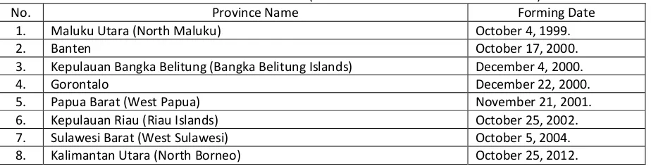
Kalimantan Utara (North Borneo) is established in 2012, while the second latest province is Sulawesi Barat (West Sulawesi) that was established in October 2004. However, the 30 provinces included in the sample are the provinces that were established prior to 2001 and not created by dividing the existing province. Thus they are well established within 2004
– 2010 research period. The name of the 6 new provinces and their forming dates is enlisted in Table 1.
Table 1. Indonesia New Provinces (After Decentralization Commencement)
No. Province Name Forming Date
1. Maluku Utara (North Maluku) October 4, 1999.
2. Banten October 17, 2000.
3. Kepulauan Bangka Belitung (Bangka Belitung Islands) December 4, 2000.
4. Gorontalo December 22, 2000.
5. Papua Barat (West Papua) November 21, 2001.
6. Kepulauan Riau (Riau Islands) October 25, 2002.
7. Sulawesi Barat (West Sulawesi) October 5, 2004.
8. Kalimantan Utara (North Borneo) October 25, 2012.
However, due to administrative issue not all of the new provinces that were formed after 1999 are having a complete data for 2004 – 2010. North Borneo does not have any data available. Additionally, there are three provinces that do not have population data; namely West Papua, Riau Islands, and West Sulawesi; thus they are also excluded from the dataset. Two provinces among the rest 30 provinces; namely Kalimantan Tengah
(Central Borneo) and Sulawesi Tenggara (South-East Sulawesi) has missing value for expenditure in 2004 that may due to incomplete reporting to the central government. Therefore, the incomplete observation (xkit; province in a certain year) that has missing value of the variables are not included in the regression and the dataset is considered to be unbalanced. However, the dataset is considered to still be representing national level because 28 provinces that are incorporated have complete observations for each year.
3.2 Data
The data were gathered from the Directorate General of Financial Balance (DGFB) the Ministry of Finance of Indonesian Republic as well as Central Statistical Agency (CSA) of the Indonesian Republic websites. The data taken from DGFB consists of
expenditures and block grants as stated in the Budget Realization Reports that are submitted annually by the local governments to DGFB. The reports are the provincial government reports. The data taken from CSA consists of Regional GDP and Population by level of both dependent and independent variables. Unfortunately, data with regards to Price Index is not available for provinces. However the Fixed Effect Panel Data Regression that is used in this research deals with endogeneity problems. The level term data was also converted into their natural log forms to implement regression analyses with regard to percentage changes.
There are four outlying observations that are being dropped from the datasets, namely the
Gorontalo and Maluku Utara (North Maluku) provinces in 2009 and 2010. Gorontalo’s value of ExpCap in 2009 and 2010 were 30.6 and 78.5 respectively while the average value of ExpCap from 2004 – 2008 is approximately 0.54. On the other
hand, the value of Maluku Utara’s ExpCap in 2009 and
average value is approximately 0.65. The value of IncCap and BGCap in 2009 and 2010 for both provinces were similarly a lot higher than the mean value of both variables within 2004 – 2008.
It is possible that both provinces receive a high level of grants within those years since they are provinces that remotely located in eastern Indonesia and rather newly formed (Maluku was formed in 1999 and Gorontalo was formed in 2000). Yet other relatively new provinces that were formed after the
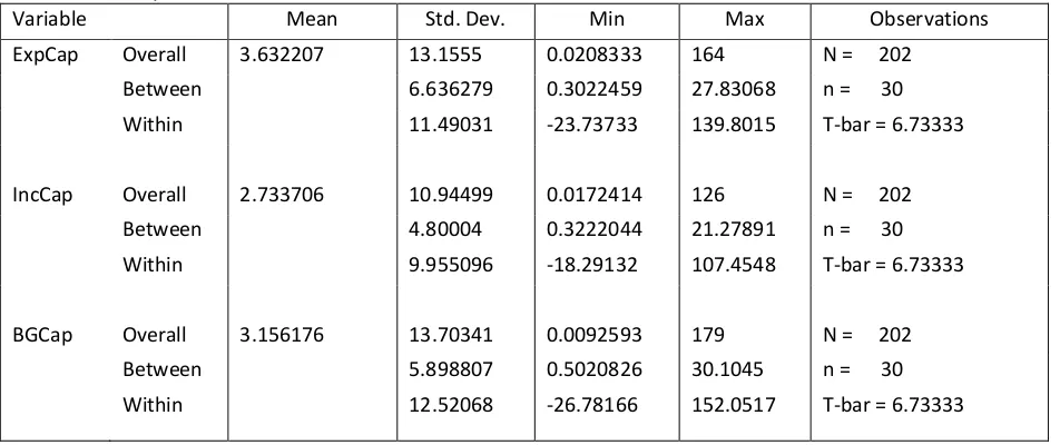
reformation era in 1999 were not receiving similar high grants. However, it is impossible for either province to experience boom in their incomes as shown in the Regional GDP values that were reflected into IncCap value. Considering there is no formal explanation of the reason behind high values, those observations were being dropped from the datasets. The summary statistics of each variable in both level and log terms are provided in Table 2.
Table 2. Summary Statistics of Variables in Level Forms
Variable Mean Std. Dev. Min Max Observations
ExpCap Overall 3.632207 13.1555 0.0208333 164 N = 202
Between 6.636279 0.3022459 27.83068 n = 30
Within 11.49031 -23.73733 139.8015 T-bar = 6.73333
IncCap Overall 2.733706 10.94499 0.0172414 126 N = 202
Between 4.80004 0.3222044 21.27891 n = 30
Within 9.955096 -18.29132 107.4548 T-bar = 6.73333
BGCap Overall 3.156176 13.70341 0.0092593 179 N = 202
Between 5.898807 0.5020826 30.1045 n = 30
Within 12.52068 -26.78166 152.0517 T-bar = 6.73333
Table 2. Summary Statistics of Variables in Level Forms (continued)
Variable Mean Std. Dev. Min Max Observations
lexpcap Overall 4.50E-09 1.439901 -3.871201 5.099866 N = 202
Between 0.9613365 -1.373279 3.171733 n = 30
Within 1.080478 -3.863492 4.696338 T-bar = 6.73333
linccap Overall -1.61E-09 1.210505 -4.060443 4.836282 N = 202
Between 0.7864787 -1.363165 2.475432 n = 30
Within 0.9201356 -3.405731 4.974185 T-bar = 6.73333
lbgcap Overall -0.0007644 1.349552 -4.682131 5.187386 N = 202
Between 0.8431895 -1.296174 2.298288 n = 30
Within 1.058419 -3.386721 5.332976 T-bar = 6.73333
3.3 Model and Method
The equation that will be estimated through the research is generally as follow:
ExpCapit = β0 + β1IncCapit + β2BGCapit + μit (3.1)
where:
ExpCapit : Local Government Expenditure per Capita IncCapit : Income per Capita
BGCapit : Block Grant per Capita μit : Residuals (μit= λt+ αi+ εit)
λt : Unobserved Time Effect αi : Unobserved Individual Effect εit : Idiosyncratic Error Term
magnitude. On the log-log terms, the model will be as propensity of naturally increasing expenditure, income, and grants throughout the years. There are two options of detrending. The first is by using ordinal variable t that represents time; t=0 for 2004 as the base year, t=1 for 2005, t=2 for 2006, up to t=6 for 2010. Then the equation will be as follow:
ExpCapit= β0+ β1IncCapit+ β2BGCapit + tt + μit (3.3)
and
ln(ExpCapit) = β0+ β1ln(IncCapit)+ β2ln(BGCapit) + tt+ μit (3.4)
The second way of detrending is by including annual dummy variables which will make the equation to be as follow: ordinal variable (t) is roughly similar to including year dummy variables. The year dummy variables can be a better proxy for detrending because they can be used to show the volatility of data throughout the years as well as the annual trend. The detailed list of variable description is provided in Table 3.
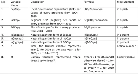
Table 3. Variable Description No. Variable
Name
Description Formula Measurement
1. ExpCapit Local Government Expenditure (LGE) per Capita of every provinces from 2004 –
3. BGCapit Block Grants per Capita of every provinces from 2004 – 2010
BG/Population in rupiah
4. ln(expcapit) Natural Logarithm form of ExpCap ln(ExpCapit) in percent 5. ln(inccapit) Natural Logarithm form of IncCap ln(IncCapit) in percent 6. ln(bgcapit) Natural Logarithm form of BGCap ln(BGCapit) in percent otherwise, dyear2 = 1 for 2005 and 0 otherwise, up to dyear7 = 1 for 2010 and 0 otherwise.
binary variable
The data will be analyzed with panel data regression of the generalized least squares both random and fixed effect methods. The robust standard error will be incorporated to fix the heteroscedasticity issue. The Hausman test will be run to investigate the probability of correlation
between the unobserved individual effect (αi) and the idiosyncratic error term (εit). From there on, it can be concluded which of the two effects is best.
Indonesia is a developing economy and before the reformation era in 1999 the country was relatively closed under the old era governance of belated former president Soeharto for about 32 years. Due to such condition, Indonesia does not have many publicly available data. Because of that it is difficult to gather data to form other control variables to be incorporated in this research. However, the fixed
effect regression method’s error term has controlled
for unobservable factors that does not change over
time (αi) therefore deals with endogeneity issue. The hypotheses that will be tested consist of: 1) Both Income per Capita and Block Grant per
Capita affects Expenditure per Capita. Null Hypothesis: H0: β1= β2 = 0
Alternate Hypothesis: H1: H0 is not true
2) The existence of flypaper effect; the difference between Income per Capita and Block Grants per Capita.
Null Hypothesis: H0: β1-β2=0
robust standard errors, by both random as well as fixed effect models to cover all of the possibilities of explanations.
4.
RESULT
Table 4 presents the regression result of level-level terms with or without trend through both random and fixed effects approaches. Subsequently, Table 5 presents similar results but with robust standard errors. For every result table, the star signs represent the level of significance of each
independent variable; with 3 stars means significant at 1% significance level (α = 1%), 2 stars means
significant at 5% significance level (α = 5%), and 1 star means significant at 10% significant level (α = 10%),
and no star means insignificant or significance level is
more than 10% (α > 10%).
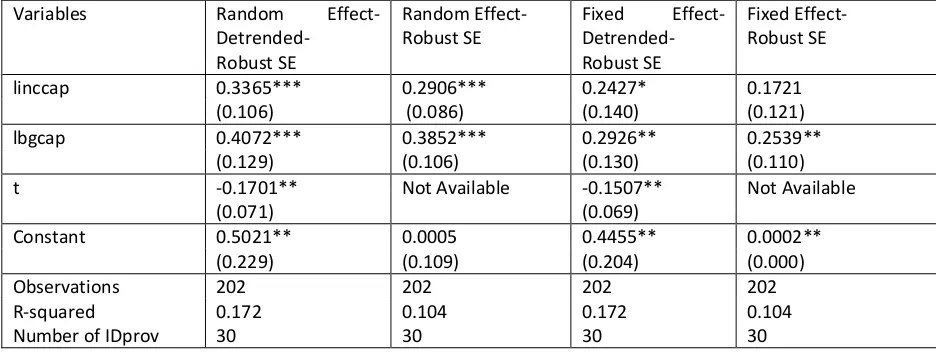
Table 6 presents the regression result of logarithm terms with or without trend through both random and fixed effects approaches. Subsequently, Table 7 presents similar results but with robust standard errors.
In testing the first hypothesis, all but one result
show that each explanatory variable affect the
dependent variable significantly although the
significance level varies across regression methods.
The only fail to reject result is the effect of linccap
towards lexpcap within fixed effect regressions with
robust standard error (Table 7). It shows that linccap does not affect lexpcap significantly. Therefore, it can
be generally concluded that both income per capita
and block grant per capita affect the expenditure per
capita and it is in line with the theory.
Table 4. Level Terms Result: with/without Trend (Dependent Variable: ExpCap)
Variables Random Effect-Detrended
Random Effect Fixed Effect-Detrended
Fixed Effect
IncCap 0.1840*** 0.1899*** 0.2035*** 0.2128***
(0.053) (0.057) (0.053) (0.057)
BGCap 0.7747*** 0.7611*** 0.7571*** 0.7402***
(0.042) (0.045) (0.042) (0.045)
t -0.3764*** Not Available -0.3755*** Not Available
(0.073) (0.120)
Constant 1.7658*** 0.6889 1.7962*** 0.7143***
(0.503) (0.455) (0.252) (0.154)
Observations 202 202 202 202
R-squared 0.976 0.972 0.976 0.972
Number of IDprov 30 30 30 30
Table 5. Level Terms Result: with/without Trend and with Robust Standard Errors (Dependent Variable: ExpCap)
Variables Random Effect-Detrended-Robust SE
Random Effect- Robust SE
Fixed Effect- Detrended-Robust SE
Fixed Effect-Robust SE
IncCap 0.1840* 0.1899* 0.2035* 0.2128
(0.100) (0.112) (0.119) (0.134)
BGCap 0.7747*** 0.7611*** 0.7571*** 0.7402***
(0.078) (0.089) (0.096) (0.110)
t -0.3764*** Not Available -0.3755*** Not Available
(0.122) (0.120)
Constant 1.7658** 0.6889 1.7962*** 0.7143***
(0.801) (0.486) (0.351) (0.082)
Table 5. Level Terms Result: with/without Trend and with Robust Standard Errors (Dependent Variable: ExpCap; continued)
Observations 202 202 202 202
R-squared 0.976 0.972 0.976 0.972
Table 6. Logarithm Terms Result: with/without Trend (Dependent Variable: lexpcap) Variables Random
Effect-Detrended
Random Effect Fixed Effect-Detrended
Fixed Effect
linccap 0.3365*** 0.2906*** 0.2427*** 0.1721*
(0.077) (0.079) (0.088) (0.089)
lbgcap 0.4072*** 0.3852*** 0.2926*** 0.2539***
(0.068) (0.070) (0.075) (0.077)
t -0.1701***
(0.041)
Not Available -0.1507*** (0.041)
Not Available
Constant 0.5021*** 0.0005 0.4455*** 0.0002
(0.155) (0.097) (0.142) (0.078)
Observations 202 202 202 202
R-squared 0.172 0.104 0.172 0.104
Number of IDprov 30 30 30 30
Table 7. Logarithm Terms Result: with/without Trend and with Robust Standard Errors (Dependent Variable: lexpcap)
Variables Random Effect-Detrended- Robust SE
Random Effect- Robust SE
Fixed Effect-Detrended- Robust SE
Fixed Effect- Robust SE
linccap 0.3365*** 0.2906*** 0.2427* 0.1721
(0.106) (0.086) (0.140) (0.121)
lbgcap 0.4072*** 0.3852*** 0.2926** 0.2539**
(0.129) (0.106) (0.130) (0.110)
t -0.1701** Not Available -0.1507** Not Available
(0.071) (0.069)
Constant 0.5021** 0.0005 0.4455** 0.0002**
(0.229) (0.109) (0.204) (0.000)
Observations 202 202 202 202
R-squared 0.172 0.104 0.172 0.104
Number of IDprov 30 30 30 30
In this dataset trend is proven to be significant
under both level and logarithm terms. The individual year dummies are mostly insignificant yet they are jointly significant. The joint significance magnitude (the F-test value) of the year dummies is similar to the ordinal trend variable (t) t-statistics value. For level terms, the year dummies are jointly significant at 1% significance level while they are significant at 5% significance level under the logarithm terms.
In addition, the coefficient estimate of trends are negative because for both level and logarithm terms the individual year dummies are showing negative trends relative to the base year (2004, the first year of the observation) which means that the dependent variables (ExpCap and lexpcap) are decreasing. However, we cannot say whether the trend is annually decreasing because the individual
year dummies significances, sign, and magnitude of the coefficient estimates vary throughout the years. Yet, due to the joint significance of trend and year dummies it is important for such variables to be included in the regressions for both level and
logarithm terms. The detrended coefficient estimates
of the level terms are higher for IncCap yet lower for BGCap relative to the coefficient estimates without trend under both random and fixed effect regressions. On the other hand, the coefficient estimates of the logarithm terms are smaller for both linccap and lbgcap relative to their coefficient estimates without trend.
Another thing to note is that the R-squared
regressions of the level terms regressions with and
without trend are 0.976 and 0.972 respectively. It
generally means that the explanatory variables within
the level terms regressions explain the variance of the
dependent variable by more than 97%, quite a high
explanatory power. In addition the difference
between the regressions with and without trend of
0.04 means that the trend variable explains the
variance of ExpCap by approximately 4%. Graph 1, 2,
3, and 4 depicts the relationship between each
independent variable and the corresponding
Graph 1. Income per Capita (IncCap) and Expenditure per Capita (ExpCap)
Graph 2. Block Grant per Capita (BGCap) and Expenditure per Capita (ExpCap)
Graph 3. Natural Logarithm of Income per Capita (linccap) and Natural Logarithm of Expenditure per Capita (lexpcap)
Graph 4. Natural Logarithm of Block Grant per Capita (lbgcap) and Natural Logrithm of Expenditure per Capita (lexpcap)
The Hausman test for random and fixed effect models significantly shows the existence of correlation between individual effect (αi) and idiosyncratic error terms (εit) for both level and logarithm terms regressions. This resulted in inconsistency of the random effect regression results thus suggested the use of fixed effect regression methods because it eliminates the endogeneity problem that requires additional control variables. Yet the Hausman test is only applicable for the regression without robust standard errors.
Regarding endogeneity, data for the price index or inflation based on provinces in Indonesia are not available. This may result in the nominal data incorporated in this research as being overstated. However, the inclusion of trend and fixed effect regressions method captured such problems. There are not many macroeconomics data available in Indonesia, especially upon provincial level, thus using fixed effect regressions is generally more appropriate in this condition.
All of the robust standard errors are higher relative to the regular standard errors counterparts and they are robust enough to alter the significance
of the explanatory variables within some methodologies. Due to the different results, it appears that the regressions without robust standard errors bear the problem of heteroskedasticity even though the use of panel data would have dealt with heteroskedasticity issue to some extent. Unfortunately, the panel data prohibit the post estimation test of heteroskedasticity existence.
The second hypothesis testing is done through
post estimation ‘test’ command in the statistical
hypothesis testing results of the level terms regressions show that the existence of flypaper effect are very significant (significant at 1% significance level).
Similar derivation can be applied towards the other level terms regressions results. For instance, the difference between the two main regressors of 0.59 from the detrended random effect regression means that 1 rupiah increase in block grant per capita has stimulatory effect towards expenditure per capita 59 cents greater than a similar 1 rupiah increase in income per capita; and the difference is very significant. However, due to the result of Hausman test it is better to use the fixed effect regressions. In addition, it is also better to use the detrended regression since the year dummy variables are jointly significant.
The fail to reject result upon logarithm regressions does not necessarily mean inexistence of flypaper effect, but could be a result of the data. Within the logarithm terms, the second hypothesis test is investigating whether the difference between coefficient estimates of linccap and lbgcap affect lexpcap significantly. The coefficient estimates of linccap and lbgcap are not directly comparable because 1% change in income per capita yields different number than 1% change in block grant per capita due to difference in the initial values the two variables. In other words if flypaper effect exist, one percentage point increase in block grant per capita will increase the expenditure per capita higher than a similar increase (one percentage point) in income per capita. As we can see from the summary statistics of the variables, the mean value of block grant per capita is higher than the mean value of income per capita. Therefore, 1% change in block grant per capita is higher than 1% change in income per capita thus they cannot be directly subtracted. When they are being subtracted, the difference becomes meaningless for it does not represent a particular number that may affect the expenditure per capita. Therefore, the insignificant result of the logarithm terms regressions is predictable.
The insignificance result of the logarithm regression terms is due to the conversion of data from level to percentage. Due to the initial value difference of the two independent variables and the
fact that conversion into logarithm smooth out the level terms data, the percentage difference between linccap and lbgcap are incomparable for they bear different level (rupiah) values. Furthermore, the smoothing out data by the logarithm terms is shown in the estimation results. As we can see in from the detrended fixed effect results in Table 6 and 7, 1% increases in income per capita increase the expenditure per capita by approximately 0.24% while a similar increase in block grant per capita increases the expenditure per capita by approximately 0.29%. The estimates infers than one percentage point increase in either income of block grant per capita will yield a roughly similar results (the difference is merely 0.05%) towards the percentage increase in expenditure per capita. Such result does not say anything about the existence of flypaper effect because each percentage change of the explanatory variables bear different rupiah values in which flypaper effect being evaluated. Yet the result of logarithm that eases up the volatility of data terms is useful in seeing the effects of each variable towards the dependent variable in a percentage terms.
Another possible explanation for the inexistence flypaper effect within the logarithm terms can be due to the fact that grants are being used to finance projects that are aimed to reduce the expenditures of the local governments. The expenditure reduce is the contrary of flypaper effect because flypaper effect has a positive relationship with increase in expenditure. The result is in line with the trend that has negative sign which means that the variable has an overall decreasing trend over the years. Therefore, even though in level terms increase in block grants per capita is more simulative than a similar increase in income per capita, due to the generally decreasing trend of expenditure the flypaper effect is shown to be inexistence.
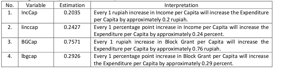
Almost all of the results are significant yet due to significance of the trend variable and result of the Hausman test, the focused of the marginal effects are those yielded from the detrended fixed effect regressions. The marginal effects of the variables are presented in Table 8. Please note that the interpretations are under the assumption that other factors are held fixed
Table 8. Marginal Effects (Fixed Effect Detrended)
No. Variable Estimation Interpretation
1. IncCap 0.2035 Every 1 rupiah increase in Income per Capita will increase the Expenditure per Capita by approximately 0.2 rupiah.
2. linccap 0.2427 Every 1 percentage point increase in Income per Capita will increase the Expenditure per Capita by approximately 0.24 percent.
3. BGCap 0.7571 Every 1 rupiah increase in Block Grant per Capita will increase the Expenditure per Capita by approximately 0.76 rupiah.
The elasticity of the mean values resulted income per capita elasticity of 0.15 and block grant per capita elasticity of 0.66 with respect to income per capita. In addition, First Difference regression analyses were also being implemented for the dataset and it yields similar results with the random effect panel data regression method.
5.
CONCLUSION
From the result, several conclusions can be taken:
1. Both Income per Capita and Block Grant per Capita affect Expenditure per Capita significantly. The correlations are positive which means that both income effect and price effect increase the expenditure of the provinces. The results are significant thus in line with the prevailing theories of the flypaper existence.
2. Block Grant per Capita affect Expenditure per Capita more than Income per Capita affect ExpCap.
From the detrended fixed effect regressions, one rupiah increase in BGCap increases the ExpCap by approximately 76 cents while 1 rupiah increase in IncCap increases ExpCap by approximately 20 cents. The difference shows that BGCap stimulates the increase in ExpCap 56 cents greater than a similar 1 rupiah increase in IncCap. It shows that BGCap affects ExpCap more than the effect of IncCap.
3. The Flypaper Effect Existed in Indonesia within 2004 – 2010.
Flypaper Effect exists under the level-level terms but undetermined under log-log terms regressions. The level terms results are very significant. It shows that increase in block grant per capita increase the expenditure per capita greater than a similar increase in income per capita. The cumulative effect will be even greater as the disparity between increase in BGCap and IncCap gets larger. The existence of flypaper
Bailey, Stephen J., and Stephen Connoly (1998), “The
Flypaper Effect: Identifying Areas for Further
Research,” Public Choice 95, 335 – 361.
Cameron, A. Colin, and Pravin K. Trivedi (2010),
Microeconomics Using Stata. Stata Press.
Courant, Paul N., et. al. 1979. “The Stimulative Effect
of Intergovernmental Grants: Or Why Money
Sticks Where it Hits”. Papers on Public
Economics. Washington D.C.: The Urban Institute.
Deller, Steven C., and Craig S. Maher (2005),
“Categorical Municipal Expenditures with a Focus on the Flypaper Effect,” Public Budgeting and Finance Fall 2005, 73 – 90.
Fisher, Ronald C. (1982), “Income and Grant Effects
on Local Expenditure: The Flypaper Effect and
Other Difficulties,” Journal of Urban Economics
12, 324 – 345.
Fisher, Ronald C. (2007), State and Local Public Finance. Thomson South-Western.
Gordon, Nora (2004), “Do Federal Grants Boost School Spending?” Journal of Public Economics
88, 1771 – 1792.
Knight, Brian (2002), “Endogenous Federal Grants and Crowd-out of State Government Spending: Theory and Evidence from the General Highway
Aid Program,” The American Economic Review
92,71 – 92.
Kusumadewi, Diah Ayu, and Arief Rahman (2007),
“Flypaper Effect pada Dana Alokasi Umum
(DAU) dan Pendapatan Asli Daerah (PAD) terhadap Belanja Daerah pada Kabupaten/Kota
di Indonesia,” (the Flypaper Effect on Block Grant and Government Own-Source Revenue towards Local Government Expenditure within Municipalities in Indonesia), Jurnal Akuntansi dan Auditing Indonesia (Indonesian Accounting and Auditing Journal) 11, 67 – 80.
Murniasih, Erny. 2006. “New Intergovernmental
Equalisation Grant in Indonesia: A Panacea or A Plague for Achieving Horizontal Balance Across
Tresch, Richard W. (2008). Public Sector Economics. Palgrave Macmillan.
Utama, Sampurna Budi, and Syahrul (2011), “Analisis
Pengaruh Unconditional Grants, Pendapatan Asli Daerah (PAD), dan Produk Domestik Regional Bruto (PDRB) terhadap Belanja Pemerintah Daerah: Studi Empiris pada
Kabupaten/Kota di Indonesia,” (The Analysis of