Inventory Control
(Production Planning & Control)
IE 2353
Pratya Poeri SuryadhiniQuantity Discount Models
Object is to Minimize total inventory costs; includes material costs
Material costs relevant in total cost: –TC = DC + D/Q(Co) + Q/2(Ch)
where
D = unit annual demand C = unit cost
Co= each order cost
Ch= carrying cost per unit per year
IC must be used in place of Chin decision-making
Steps for Solving Quantity Discount
1.
Compute EOQ for each discount price:
2.
If EOQ < discount minimum level, make Q = minimum.
3.
For each EOQ, compute total cost:
TC = DC + D/Q(Co) + Q/2(Ch)
4.
Choose the lowest cost quantity from all levels.
Q
*2DC
IC
oQuantity Discount Models
Text example:
Quantity Discount Schedule
Material cost:
•Total material cost is affected by the Discount (%)
•Unit cost if first $5.00, then $4.80, and finally $4.75
Quantity Discount Models
Total Cost Curves for each of the 3 discount plans
Figure 6.7
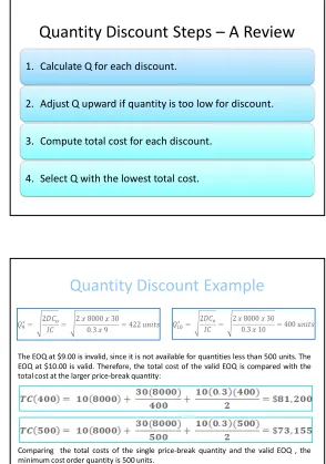
Quantity Discount Steps
–
A Review
1. Calculate Q for each discount.
2. Adjust Q upward if quantity is too low for discount.
3. Compute total cost for each discount.
4. Select Q with the lowest total cost.
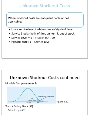
Quantity Discount Example
The Smith company purchases 8000 units of a
product each year. The supplier offers the units for
sale at $10.00 per unit for orders up to 500 units and
at $9.00 per unit for orders of 500 units or more.
What is the economic order quantity if the order
cost is $30.00 per order and the holding cost is 30%
of per unit cost per year?
Quantity Discount Example
The EOQ at $9.00 is invalid, since it is not available for quantities less than 500 units. The EOQ at $10.00 is valid. Therefore, the total cost of the valid EOQ is compared with the total cost at the larger price-break quantity:
Economic Production Quantity
The assumptions that the entire orders is received into inventory at one time (instantaneously is often not true.
The EPQ assumes continuous gradual additions to stock (finite replenishment rate) over the production period.
The EPQ formula is obtained:
p= production rate
d = demand rate
Economic Production Quantity
Economic Production Quantity
Optimum length of production run
Production reorder point in units
Total annual cost = production cost + setup cost + holding cost
EPQ Example
EPQ Example
The Use of Safety Stock
Stock-outs occur when there are uncertainties with: - Demand
- Lead time
Safety stock is extra stock on hand to avoid stock-outs
•ROP = d*L + SS
•d = average daily demand
•L = average lead time, time for an order to be delivered
•SS = safety stock
ROP is adjusted to implement safety stock policy:
The Use of Safety Stock
In
Fig. 6.8. The Use of Safety Stock
The Use of Safety Stock and ROP
Known stock-out costs:
•
Given probability of demand, find total cost for each
safety stock alternative
Unknown stock-out costs:
Known Stock-out Costs
• ABCO example:
Table 6.2
Initial calculations: ROP = 50 (d*L) Ch= $5
Css= $40/ unit (stock-out cost) D/Q = 6 times per year
Known Stock-out Costs continued
• ABCO example: Table 6.3
Calculation the EMV (expected monetary value) for each ROP
alternative
Known Stock-out Costs continued
ABCO example:
Calculations for a given ROP, N: 1. Being Short: D(S) = (N-S)* Css*D/Q,
• where S = demand during lead time 2. Being Over: D(O) = (D-O)* Ch
• where O = demand under ROP Calculations for an ROP of 40:
• Being Over
D(30) = (40-30)*$5 = $50 D(40) = $0
• Being Short
D(50) = (50-40)*$40*6 = $2,400 D(60) = (60-40)*$40*6 = $4,800 D(70) = (70-40)*$40*6 = $7,200
Known Stock-out Costs continued
ABCO example:
Last step for ROP = 40 is to calculate the EMV:
EMV = P(D) * Cost of Being Short/Over
EMV(40) =
Unknown Stock-out Costs
When stock-out costs are not quantifiable or not
applicable:
•
Use a service level to determine safety stock level.
•
Service Stock: the % of time an item is out of stock.
•
Service Level = 1
–
P(Stock-out), Or
•
P(Stock-out) = 1
–
Service Level
Unknown Stock-out Costs continued
Hinsdale Company example:
1. Lead time demand ~N(350, 10) where = 350, = 10
2. Desired Policy: P(Stock-out) = 5%
Therefore, service level = 95%
Visualization of Desired Inventory Policy:
Figure 6.9
Unknown Stockout Costs continued
Hinsdale Company example:
X = + Safety Stock (SS) SS = X – = Z
Z = =
23
Figure 6.10
X-
SS
Unknown Stock-out Costs continued
Hinsdale Company example:
Find Z using a Normal table, like in Appendix A: Z = 1.65 for a 5% right tail
Rewrite equation: Z = 1.65 = =
Solving for SS yields 16.5, or 17, units. Therefore, ROP = 350 + 17 = 367
24
Service Level versus Carrying Costs
Figure 6.11
The following curve depicts the tradeoff between carrying costs and service level for the previous example
such dramatic tradeoffs exist for all similar problems
ABC Analysis
ABC analysis divides on-hand inventory into three classifications on the basis of dollar (TL) volume.
It is also known as Pareto analysis. (which is named after principles dictated by Pareto).
The idea is to focus resources on the critical few and not on the
trivial many.
(Annual Dollar Volume of an Item) = (Its Annual Demand) x (Its Cost per unit)
ABC Analysis
Class
A
items are those on which the annual
dollar volume is high.
They represent 70-80% of total
inventory costs, but they account
for only 15% of total inventory
items.
ABC Analysis
Class
B
items are those on which
annual dollar volume is medium.
They represent 15-25% of total
dollar value, and they account for
30% of total inventory items on the
ABC Analysis
Class
C
items are low dollar volume
items.
They represent only the 5% of total
dollar volume, but they include as
many as 50-60% of total inventory
items.
ABC Analysis
ABC Analysis
Some of the Inventory Management Policies that may be based on ABC analysis include:
a) Class A items should have tighter inventory control.
b) Class A items may be stored in a more secure area.
c) Forecasting Class A items may warrant more care.
Summary of ABC Analysis
•
Group A Items - Critical
•
Group B Items - Important
•
Group C Items - Not That Important
32
ABC Inventory Analysis
0
Percent of Inventory Items
P
ABC Inventory Policies
34
Greater expenditure on supplier development
for A items than for B items or C items
Tighter physical control on A items than on B
items or on C items
Greater expenditure on forecasting A items
than on B items or on C items
ABC Inventory Example
Item Unit cost Annual Usage
Annual Dollar Usage
Total Annual Persentage Usage
1 0.05 50000 2500 34.3
2 0.11 2000 220 3.0
3 0.16 400 64 0.9
4 0.08 700 56 0.8
5 0.07 4800 336 4.6
6 0.15 1300 195 2.7
7 0.20 17000 3400 46.7
8 0.04 300 12 0.2
9 0.09 5000 450 6.2
10 0.12 400 48 0.6
ABC Inventory Example
Rank by percentage of usageItem Annual Dollar Usage Total Annual Persentage Usage Cumulative Percentage Item Classification
Rank by Classification
Item Classification Items Percentage Percentage Value
A 7, 1 20 81
B 9, 5, 2, 6 40 16.5