Compressive Adaptation of Large Steerable Arrays
Dinesh Ramasamy, Sriram Venkateswaran, Upamanyu Madhow
Department of Electrical and Computer Engineering
University of California, Santa Barbara, CA 93106, USA
Abstract—We consider the problem of adapting very large antenna arrays (e.g., with 1000 elements or more) for tasks such as beamforming and nulling, motivated by emerging applications at very high carrier frequencies in the millimeter (mm) wave band and beyond, where the small wavelengths make it possible to pack a very large number of antenna elements (e.g., realized as a printed circuit array) into nodes with compact form factors. Conventional least squares techniques, which rely on access to baseband signals for individual array elements, do not apply. Hence the preferred approach is to perform radio frequency (RF) beamsteering, with a single complex baseband signal emerging from a receive array, or going into a transmit array. Further, we are interested in what can be achieved with coarse-grained control of individual elements (e.g., four-phase, or even binary phase, control). In this paper, we propose an adaptation architecture matched to these hardware constraints. Our approach comprises the following two steps. The first step is compressive estimation of a sparse spatial channel using a small number of measurements, each using a different set of randomized weights. However, unlike the standard compressive sensing formulation, we are interested in estimating continuous-valued parameters such as the angles of arrivals of various paths. The second step is quantized beamsteering, where weights for beamforming and nulling, subject to the constraint of severe quantization, are computed using the channel estimates from the first step. We provide promising preliminary results illustrating the efficacy of this approach.
I. INTRODUCTION
We begin with the following question: how does one effec-tively adapt a very large array (e.g., 1000 elements or more) for tasks such as beamforming and nulling, while accounting for natural hardware constraints? The motivating application is communication using very high carrier frequencies in the millimeter (mm) wave band and beyond, where the small wavelengths make it possible to pack a very large number of antenna elements (e.g., realized as a printed circuit array) into nodes with compact form factors. Using a separate RF chain for each antenna element is out of the question in such settings, hence it is not possible to employ standard least squares style adaptation, which requires access to the complex baseband signal corresponding to each antenna element. Thus, we limit ourselves to RF beamforming: at the transmitter, a single com-plex baseband waveform is upconverted to RF and distributed to the antenna elements, with digital control of the amplitude and phase of each element; at the receiver, the RF signals at different elements are combined after digitally controlling the
This work was supported by the National Science Foundation through the grant CNS-0520335, and by the Institute for Collaborative Biotechnologies through the grant W911NF-09-0001 from the U.S. Army Research Office. The content of the information does not necessarily reflect the position or the policy of the Government, and no official endorsement should be inferred.
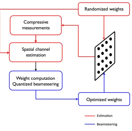
Fig. 1. Architecture to adapt large steerable arrays with coarse control: Explicit estimation of the steering direction using a few random projections, followed by beamsteering with only four phases.
amplitude and phase at each element, and downconverted to obtain a single complex baseband waveform.
Approach and Summary of Results: In this paper, we
propose a new approach for adapting large arrays, shown in Figure 1, comprising the following steps. The first step is compressive estimation, in which a small set of measure-ments using RF beamforming with pseudorandom weights are employed for estimation of continuous-valued parameters characterizing a sparse spatial channel. However, rather than employing the inherently discrete ℓ1 optimization framework
of standard compressive sensing, we employ a version of orthogonal matching pursuit to obtain coarse estimates of the spatial frequencies, followed by sequential Newton re-finements that provide accuracies far better than would be possible by optimizing over a discrete grid. The second step isquantized beamsteering,in which these explicit channel es-timates are employed for computing weights for beamforming and nulling, subject to the severe quantization (e.g., phase-only control with a small number of phases). Starting with an unquantized zero-forcing solution, we show that sequential optimization provides effective solutions for heavily quantized weights.
comprehensive system design and performance evaluation left for future work. For example, we abstract out the cross-layer protocols and low layer signal processing (e.g., correlation against training sequences, compensating for carrier offsets) required to implement compressive estimation. For quantized beamsteering, we consider the problem of steering one beam and a few nulls, without specifying whether the nulls corre-spond to undesired multipath or interference. A number of interesting theoretical issues require further investigation, as discussed in the conclusions.
Related work: Our approach of explicitestimation followed
by weight computation is a stark contrast toimplicitadaptation using classical least squares techniques. It also differs from recent codebook-based approaches to 60 GHz RF beamform-ing [1], [2]. The latter do not, for example, provide enough information for interference suppression. An alternative ap-proach for implicit adaptation, which could potentially provide beamforming as well as interference suppression gains, is randomized linear ascent, proposed by Widrow and McCool more than three decades ago [3]. However, this algorithm does not scale to large arrays (at least not for rapid initial training), since its convergence time is proportional to the square of the number of array elements. The millimeter wave channel is quite sparse, with the number of dominant multipaths being small compared to the large number of array elements of interest to us (e.g., see [4], [5] for modeling of outdoor 60 GHz links). It is therefore natural to invoke ideas from compressive sensing [6]–[9], where a signal which is sparse with respect to a fixed basis, is reconstructed (e.g., using ℓ1
optimization) from projections onto a small number of vectors that are “incoherent” with respect to the original basis, in terms of satisfying the so-called restricted isometry property (RIP). Roughly speaking, RIP means that the most of the energy of the sparse signal is captured by these “compressive measure-ments.” In our compressive estimation approach, we leverage the first part of the compressive sensing framework, in terms of capturing the required information using a small number of measurements. However, standard ℓ1 reconstruction does not
work well under basis mismatch [10] (e.g., for estimation of a continuous-valued frequency using a DFT basis), hence it is necessary to develop alternative techniques for estimating continuous-valued parameters. Theoretical frameworks for the latter are emerging [11], [12], but their implications for spe-cific scenarios, and the development of effective algorithms, requires further work. In particular, our problem of spatial frequency estimation maps exactly to the standard frequency estimation problem recently revisited by Duarte and Baraniuk in a compressive setting [13]. We are, however, interested in both one- and two-dimensional frequencies (corresponding to linear and two-dimensional antenna arrays), and our Newton-based technique provides more refined estimates than the grid-based algorithm in [13]. Also, we are ultimately interested not just in the abstract problem of spatial frequency estimation, but also in cross-layer designs for beamsteering which use it as a building block.
Prior work related to our approach to quantized
beam-steering includes [14], [15]. A naive approach is to compute complex-valued weights without quantization constraints, fol-lowed by scalar quantization of each weight; however, this does not perform well with drastic quantization. In [14], it was shown that sequential update of quantized weights can be used to obtain effective interference suppression. We use similar ideas here, although our goal now is a multiobjective cost func-tion including both beamforming and nulling. Beamforming patterns for large arrays with heavily quantized weights have been explored recently in [15], but direct optimization of cost functions related to communication goals is not considered there.
Outline: The system model is described in Section II along
with an overview of our solution. Section III contains a detailed description of our compressive estimation algorithm, and provides numerical results showing its efficacy. Section IV describes our approach to quantized beamsteering in detail, and provides example numerical results that illustrate both its effectiveness and its suboptimality. Finally, Section V contains our conclusions.
II. SYSTEMMODEL ANDOVERVIEW
Consider a uniformdspaced linear array withN elements. Typical values of interest are d=λ/2 ord=λ/3, where λ
denotes the carrier wavelength. For angle of arrival (AoA)θ, the normalized array response is given by
a(ω) = (1, ejω, ej2ω, . . . , ej(n−1)ω)T/√N ,
(1)
whereω= 2πdsinθ/λis the correspondingspatial frequency. Thus, AoA estimation can be equivalently viewed as estima-tion of spatial frequency. For a multipath channel with K
dominant paths, the net array response is a linear combination of the form:
anet = k=K
!
k=1
gka(ωk), (2)
wheregk denotes the complex amplitude of the kth multipath
component, andωk, its spatial frequency.
Our goal is to estimate{gk, ωk}usingM measurements of
the form:
yi=wTi anet+zi i= 1,2, . . . , M,
where wi are the receive beamforming weights and zi is
the measurement noise. Implementation considerations with large arrays restrict the entries of wi to a small set: for
example, to two bits of phase precision, with entries chosen from{±1,±j}. Concatenating the measurements, we get
y=WTanet+z, (3)
whereW= [w1w2 . . . wM].
We begin with the following question: given that the number of AoAs K is much smaller than the number of antenna elements N, can we reduce the number of measurementsM
multiples of 2π/N. In this case, anet can be expressed as a
linear combination of the columns of
A=
Kentries ofxare nonzero, since there are onlyKAoAs. The observationsycan be written as
y=WTAx+z. (5)
By substituting (1) in (4), we observe that the matrix A is the Discrete Fourier Transform (DFT) matrix. Since the DFT matrix is orthonormal, standard Compressive Sensing theory guarantees that with (a) measurements of the form (5), (b) the elements of W chosen i.i.d. from a class of distributions (including the Bernoulli distribution) and (c) the number of measurementsM =O(KlogN),x(and thus the spatial frequencies) can be recovered with high probability. This suggests that when the spatial frequencies come from the DFT grid, roughly KlogN ($N) measurements, with the beamforming weightsWchosen i.i.d. from{±1,±j}, suffice to estimate them.
However, in reality, the spatial frequencies ωk are not
restricted to integer multiples of 2π/N and come from a continuum. We could ignore this fact and apply standard CS recovery algorithms assuming that spatial frequencies are integer multiples of2π/N. However, this limits the estimation accuracy to the spacing between the frequencies (even when we oversample the frequencies). We now outline our approach for overcomeingthis problem.
First, we estimate the AoAs coarsely by quantizing the spatial frequencies to integer multiples of 2π/R (R ≥ N)
and then applying a variant of orthogonal matching pursuit to obtain coarse estimates of {ωm}. These estimates are further
refined using Newton-style local search; this is inspired by recent work [16] showing that Newton-based approaches are very effective in attaining fundamental bounds on timing estimation in a classical setting. We describe the algorithm in detail in Section III.
Quantized Beamsteering:Each node can use the compressive
estimation algorithm outlined above on a slow time scale to track the spatial channel to/from each of its neighbors. It can then use these estimates to steer its beam towards a desired communication partner, while steering nulls towards other neighbors and undesired multipath components. Our compressive estimation framework does not require tight am-plitude and phase control for the array elements. Thus, an important question is whether we can also perform tasks such as beamforming and nulling with such coarse control of array elements. We explore this in Section IV.
We begin with a standard zero-forcing solution, whose phases are quantized to the available alphabet. This is then refined by a sequential update process as in [14]. We are unable to make any claims of optimality at this point, and simply provide illustrative numerical results which show that we can effectively utilize a large array with phase-only control.
III. COMPRESSIVEESTIMATION
In this section, we describe an algorithm to estimate multi-ple spatial frequencies using compressive measurements from an array. We assume that the number of frequencies K is known. The algorithm has two stages: first, we discretize the set of frequencies[0,2π] and use a variant of the traditional Orthogonal Matching Pursuit (OMP) to coarsely estimate the
K frequencies on the discrete grid. We then refine each fre-quency sequentially using Newton’s method. For simplicity of exposition, we first discussion estimation of a single frequency. We then use these ideas as building blocks in developing an algorithm to estimateK frequencies.
DefineS(ω) to be WTa(ω), ω
∈[0,2π]; theith entry of S(ω) is the DTFT of wi evaluated at ω. The measurement
model in (3) reduces to
y= K !
k=1
gkS(ωk) +z. (6)
Single Frequency: When there is only one frequency, the
measurementsyare given by
y=g1S(ω1) +z, (7)
where the noisez∼CN(0, σ2I M).
The estimation procedure is built on the following observa-tion: the generalized likelihood ratio test (GLRT) estimate of
ω1, treating the unknown gain g1 as a nuisance parameter,
is the frequency at which the normalized array response S(ω)/||S(ω)||correlates best with the observationsy:
The first step is to estimate ω1 coarsely by picking the
maximum of the cost functionJ(ω)from among R discrete frequencies{0,2π
R, . . . ,
2π(R−1)
R }. Here,Ris typically chosen
at least as large as the number of antenna elementsN. Next, we refine the coarse estimate by using Newton’s method to optimize the cost function J(ω). Let us denote the estimate of ω1 in the ith iteration of Newton’s method
byωˆ1(i). Starting off atωˆ (i)
1 , an additional Newton refinement
step produces the estimateωˆ1(i+1), given by
≥ 0. We therefore use (9) to refine the estimate only whenJ(ω)is concave atωˆ1(i).
When the function is convex atωˆ1(i), we use the following
observation to design an alternate refinement rule: if the GLRT estimate ωˆ1 in (8) is close to the true frequency ω1 (“reasonable” number of measurements and noise), then
function J(ˆω1) ≈ ||y2||. Therefore, to get closer to the
optimum, we design a Newton step that solvesJ(ω) =||y||2. This gives us the update rule
ˆ
ω(1i+1)= ˆω(1i)+'
y'2−J)ωˆ1(i)
*
J")ωˆ(i)
1
* . (10)
Multiple Frequencies: When there is more than one
fre-quency to be estimated, we use each part of the algorithm described above recursively. However, there is one key modi-fication: while estimating thelth frequencyωl, we project out
the contributions from the frequencies that we have already estimated to the observations y (and also the template S(ω)
for the refinement stage), thereby roughly reducing it to a single frequency problem at each stage. We briefly describe the coarse estimation and the Newton refinement steps.
Coarse estimation: Suppose that we have estimated l−1
frequencies ωˆ1,ωˆ2, . . . ,ωˆl−1 coarsely. The contribution from
these frequencies to the observationsylies in the span of the matrix
B=+
S(ˆω1) S(ˆω2) . . . S(ˆωl−1) ,.
Thus, we can eliminate these contributions by operating on the observations y with the orthogonal projection matrix B⊥ =
I− B(BH
B)−1BH
to obtain the residual vector,
rl−1=B⊥y.
We now pretend that thelth frequencyωlis the only one left in
rl−1and estimate it exactly as in the single frequency setting:
by sampling the function
Jl(ω) = &
&rHl−1S(ω) & &
2
'S(ω)'2
at {0,2π R, . . . ,
2π(R−1)
R }, R ≥N and picking the maximum.
We denote this estimate by ωˆl, add it to the set of estimated
frequencies and continue with the coarse estimation procedure until we estimate K frequencies.
Newton refinement: We refine our estimates of the K fre-quencies by applying Newton’s method to them sequentially. The refinement process for each frequency is very similar to the single frequency case; the only difference is that the contributions from the other frequencies are projected out (from both yandS(ω)) while defining the cost function.
Suppose that at some stage of the refinement process, our estimates of the K frequencies are given by ωˆ1,ωˆ2, . . . ,ωˆK
respectively and we want to further refine the lth frequency. Just as before, the contributions from the otherK−1 frequen-cies can be eliminated from the observations y by using the orthogonal projection matrixH⊥, which is obtained from
H=+
S(ˆω1) . . . S(ˆωl−1) S(ˆωl+1) . . . S(ˆωK) ,
as H⊥=I− H(HH H)−1
HH. The residual is given by
H⊥y
and we denote this byyl. Assuming that theK−1frequency
estimates are reasonably good, we have,
yl≈glH⊥S(ωl) + ˜z
This resembles the model (7) for single frequency estimation. We can therefore use the Newton updates specified before to refine ωˆl by replacingy withyl andS(ω) withH⊥S(ω) in
the definition of the cost function (8), (9) and (10).
One round of Newton updates consists of applying the above refinements to each of theKfrequencies, and we run multiple such rounds.
Results: We begin by simulating the problem of estimating
K = 2 spatial frequencies with an N = 32 element array, with the elements spaced λ/2 apart. We find that M = 12
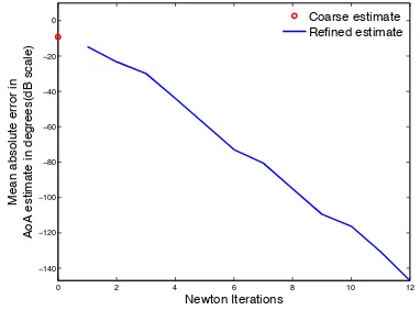
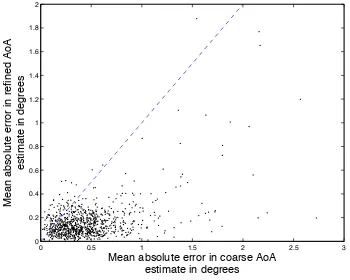
measurements typically suffice to estimate the two AoAs. Figure 2 shows that, in the absence of measurement noise, the proposed Newton refinements improve the estimates of the spatial frequencies to any desired accuracy. Figure 3 is a scatterplot of the estimation errors before and after refinement in the presence of measurement noise over 1000 trials. We see that the errors after refinement are considerably smaller (most of them lie well below the line with slope 1 shown in blue). For this scenario, the algorithm succeeds in 96% of the trials (failures are due to gross errors in the coarse estimation stage) and the Newton refinements improve the median estimation error from 0.4015◦to0.1376◦.
0 2 4 6 8 10 12
−140
−120
−100
−80
−60
−40
−20 0
Newton Iterations
Mean absolute error in
AoA estimate in degrees(dB scale)
Coarse estimate Refined estimate
Fig. 2. 10 log10(Average AoA error)is plotted as a function of refinement
rounds. We takeM= 12noiseless measurements from aN= 32element
λ/2spaced array whenK= 2beams impinge the antenna array. A coarse estimate of the frequencies is made using a4N= 128grid.
To illustrate that we need significantly fewer measurements than the number of elements N as the array gets larger, we consider the problem of estimating K = 2 spatial frequen-cies(one at 12dB and another at 9dB) from a linear array
of N = 1024 elements spaced λ/2 apart. We find that
M = 24measurements (only2.3%of the number of elements) suffice to estimate the two AoAs, with the refinement process improving the median error from9.6◦×10−3to2.7◦×10−3.
0 0.5 1 1.5 2 2.5 3 0
0.2 0.4 0.6 0.8 1 1.2 1.4 1.6 1.8 2
Mean absolute error in coarse AoA estimate in degrees
Mean absolute error in refined AoA
estimate in degrees
Fig. 3. Comparison of AoA estimation errors in the presence of noise before and after refinements of the spatial frequencies.M= 12measurements made from aN= 32elementλ/2spaced array whenK= 2beams, one at12dB and another at9dB fall on the array.4N= 128grid points used to arrive at the coarse estimates. The blue dashed line is the slope one line.
IV. QUANTIZEDBEAMSTEERING
The AoA estimates from Section III give us the directions in which we need to steer transmissions and place nulls (to combat multipath or avoid interference). However, hardware design imposes severe constraints: we would like to steer beams by only changing the antenna phases that are heavily quantized (say, to two bits of precision). We now explain how we can do this effectively.
Consider a two dimensional square array consisting of N
(typically32×32 = 1024) elements. The separation between the elements along either side is d. Denoting the transmit gain and phase at the (m, n)th element by gmn and βmn
respectively, the received power at an azimuthφand elevation
θ is given by
P =
& & & & &
!
m,n
gmnejβmnexp (j(mωx+nωy))
& & & & &
2
, (11)
whereωx= (2πd/λ) sinθcosφandωy = (2πd/λ) sinθcosφ
are the spatial frequencies associated with the elevation and azimuth. For convenience, we denote the combined spatial frequencies (ωx, ωy)byω and the power at ωbyP(ω).
Our goals are twofold: (a) The received power in the direc-tion of intended receiver P(ω0)must be as high as possible.
(b) The interference caused in Qother directions (these may represent other users or undesired multipath components), given by P(ωi), i= 1, . . . , Q, must be as small as possible. We try to achieve these goals simultaneously by maximizing the signal-to-nullratioγ, given by
γ= P(ω0)
-Q
i=1P(ωi)
. (12)
We abstract the hardware constraints as follows: (a) The gains gmn are fixed once and for all to a two dimensional
Chebyshev window (in order to control undesired sidelobes). (b) The phase shiftsβmn which we use to steer the
transmis-sion can only take one of the four values{±1,±j}.
Before describing our approach, we introduce some nota-tion. We separate the terms in (11) into the phases that we con-trol and the rest that are fixed. Letψbe a vectorized version of the phases[ejβmn]
anda(ω)be the corresponding vectorized version of the steering matrix [gmnexp (−j(mωx+nωy))].
Then the powerP(ω) =&
&a(ω)Hψ & &
2
. We also denote thelth entry of ψ byψ[l].
The basic idea behind our algorithm is as follows: given a feasible solution for the phasesψ, we can improve it with low-complexity until we settle at a local optimum. To see this, note thatψ[l]takes only one of four values{±1,±j}. Therefore, given the phases at the other elements, we can easily find which of these choices forψ[l] maximizesγ: hold the other phases fixed, try out each of the four phases in thelth position ofψ, use (12) to computeγfor each of these candidates and pick the maximum. Let us denote the maximizing phase by
α∗∈ {±1,±j}. Ifψ[l]is different fromα∗, we can improve the solution by simply replacing ψ[l] withα∗. By repeating this procedure for different choices of l, we can improveγ, without ever lowering it, until we settle at a local optimum. We refer to the phases at the end of this procedure as the sequentially optimized phases.
Since the powers are computed at specific frequencies in (12), the solution thus obtained could be sensitive to the errors in estimating these frequencies from Section III. To reduce this sensitivity, we replace the metricγwith a modified versionγ˜, where the powers are computed in a small band around each frequencyωi, i= 0,1, . . . , Q:
˜
γ= .
P(ω0−h)dh
-Q
i=1
.
P(ωi−h)dh
.
The width of the band (the region of integration) is dictated by the estimation error in Section III.
Initialization:The only thing that we need to specify now is a starting point that is both feasible and “reasonably good” (so that we do not settle at a bad local optimum). We compute the starting point by relaxing the constraints on the entries of ψ, allowing them to take any value whatsoever. We can now cast our problem as a standard zero-forcing problem of choosing weights to null out transmissions inQdirections per-fectly, while maximizing the power in the intended direction. Specifically, we solve:
maximize |a(ω0)Hψ|
subject to 'ψ'= 1
a(ωi)Hψ= 0 ∀i∈ {1,2, . . . Q}
We then quantize these phases to the closest among
{±1,±i}, thus giving us a feasible solution to the problem that is also reasonably good. We term these phases the na¨ıvely quantized phases and use them to initialize our sequential optimization procedure.
Results: We steer the transmission towards a receiver while
simultaneously placing nulls inQ= 2directions, using a 32
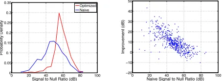
optimized phases. We see thatγis tightly clustered around its mean value of 58 dB for the sequentially optimized phases. The na¨ıvely quantized phases have a lower γ on the average (48 dB) and also exhibit greater variance.
Figure 4(b) plots the gains provided by sequential optimiza-tion against the signal-to-null ratio obtained with the na¨ıvely quantized phases. We see that the improvements are large when naive quantization does poorly and decrease as naive quantization become better. Thus, the sequential optimization procedure gives us the largest gains exactly when we need them.
0 20 40 60 80 100 0
0.05 0.1 0.15 0.2 0.25 0.3 0.35
Signal to Null Ratio (dB)
Probability Density
Optimized Naive
(a) Histogram of γ optimized(red) and na¨ıvely quantized(blue) phases
0 20 40 60 80 100
−20
−10 0 10 20 30 40 50
Naive Signal to Null Ratio (dB)
Improvement (dB)
(b) Improvements provided by se-quential optimization plotted against the na¨ıve signal to null ratio
Fig. 4. Results for quantized beamsteering with a32×32element array
with the elements placed λ/2apart. We place Q= 2nulls while steering transmissions towards a receiver.
V. CONCLUSIONS
The preliminary results in this paper show the feasibility of our approach to compressive adaptation of large arrays with drastically simplified hardware control: the architecture can be realized using RF beamsteering with coarse-grained control of the phases of the array elements. The proposed approach of explicit estimation and weight computation differs fundamentally from implicit adaptation using classical least squares, which is incompatible with RF beamforming, as well as from codebook-based techniques, which enable coarse beamforming but not nulling.
An important topic for future work is the design of cross-layer protocols and signal processing for compressive adap-tation in specific settings of interest, such as for packetized 60 GHz backhaul mesh networks [17]. At a fundamental level, it is important to develop a theoretical understanding of the limits of compressive estimation of continuous-valued parameters, as well as algorithms for attaining these limits. This problem has received far less attention than the “discrete” compressive sensing problem. Similarly, we would like to develop a theoretical understanding of the limits of quantized beamsteering, as well as improved algorithms for computing optimal or near-optimal solutions at reasonable complexity.
Acknowledgements
This work was informed and motivated by discussions with Prof. Mark Rodwell on large arrays and the associated hardware constraints.
REFERENCES
[1] J. Wang, Z. Lan, C. woo Pyo, T. Baykas, C. sean Sum, M. Rahman, J. Gao, R. Funada, F. Kojima, H. Harada, and S. Kato, “Beam code-book based beamforming protocol for multi-gbps millimeter-wave wpan systems,”Selected Areas in Communications, IEEE Journal on, vol. 27, no. 8, pp. 1390 –1399, october 2009.
[2] S. Lin, K. Ng, H. Wong, K. Luk, S. Wong, and A. Poon, “A 60ghz digitally controlled rf beamforming array in 65nm cmos with off-chip antennas,” inRadio Frequency Integrated Circuits Symposium (RFIC), 2011 IEEE, june 2011, pp. 1 –4.
[3] B. Widrow and J. McCool, “A comparison of adaptive algorithms based on the methods of steepest descent and random search,”Antennas and Propagation, IEEE Transactions on, vol. 24, no. 5, pp. 615 – 637, sep 1976.
[4] H. Zhang, S. Venkateswaran, and U. Madhow, “Channel modeling and MIMO capacity for outdoor millimeter wave links,” in Proc. IEEE WCNC 2010, April 2010.
[5] H. Zhang and U. Madhow, “Statistical modeling of fading and diversity for outdoor 60GHz channels,” in Proc. International Workshop on mmWave Communications (mmCom 2010), September 2010.
[6] E. Candes, J. Romberg, and T. Tao, “Robust uncertainty principles: exact signal reconstruction from highly incomplete frequency information,”
Information Theory, IEEE Transactions on, vol. 52, no. 2, pp. 489 – 509, feb. 2006.
[7] E. Candes and T. Tao, “Near-optimal signal recovery from random projections: Universal encoding strategies?” Information Theory, IEEE Transactions on, vol. 52, no. 12, pp. 5406 –5425, dec. 2006. [8] ——, “Decoding by linear programming,” Information Theory, IEEE
Transactions on, vol. 51, no. 12, pp. 4203 – 4215, dec. 2005. [9] D. Donoho, “Compressed sensing,”Information Theory, IEEE
Transac-tions on, vol. 52, no. 4, pp. 1289 –1306, april 2006.
[10] Y. Chi, L. Scharf, A. Pezeshki, and A. Calderbank, “Sensitivity to basis mismatch in compressed sensing,”Signal Processing, IEEE Transactions on, vol. 59, no. 5, pp. 2182 –2195, may 2011.
[11] M. Duarte and Y. Eldar, “Structured compressed sensing: From theory to applications,” Signal Processing, IEEE Transactions on, vol. 59, no. 9, pp. 4053 –4085, sept. 2011.
[12] T. Blumensath and M. Davies, “Sampling theorems for signals from the union of finite-dimensional linear subspaces,”Information Theory, IEEE Transactions on, vol. 55, no. 4, pp. 1872 –1882, april 2009.
[13] M. Duarte and R. Baraniuk, “Recovery of frequency-sparse signals from compressive measurements,” in Communication, Control, and Computing (Allerton), 2010 48th Annual Allerton Conference on, 29 2010-oct. 1 2010, pp. 599 –606.
[14] O. Bakr, M. Johnson, R. Mudumbai, and U. Madhow, “Interference suppression in the presence of quantization errors,” inCommunication, Control, and Computing, 2009. Allerton 2009. 47th Annual Allerton Conference on, 30 2009-oct. 2 2009, pp. 1161 –1168.
[15] C.-P. Yeang, G. Wornell, and L. Zheng, “Oversampling transmit and receive antenna arrays,” in Acoustics Speech and Signal Processing (ICASSP), 2010 IEEE International Conference on, march 2010, pp. 2522 –2525.
[16] P. Bidigare, U. Madhow, R. Mudumbai, and D. Scherber, “Attaining fundamental bounds on timing synchronization,” inIEEE International Conference on Acoustics, Speech, and Signal Processing (ICASSP 2012), Kyoto, Japan, March 2012, to appear.