Abstract—Image Compression using Artificial Neural Networks is a topic where research is being carried out in various directions towards achieving a generalized and economical network. Feedforward Networks using Back propagation Algorithm adopting the method of steepest descent for error minimization is popular and widely adopted and is directly applied to image compression. Various research works are directed towards achieving quick convergence of the network without loss of quality of the restored image. In general the images used for compression are of different types like dark image, high intensity image etc. When these images are compressed using Back-propagation Network, it takes longer time to converge. The reason for this is, the given image may contain a number of distinct gray levels with narrow difference with their neighborhood pixels. If the gray levels of the pixels in an image and their neighbors are mapped in such a way that the difference in the gray levels of the neighbors with the pixel is minimum, then compression ratio as well as the convergence of the network can be improved. To achieve this, a Cumulative distribution function is estimated for the image and it is used to map the image pixels. When the mapped image pixels are used, the Back-propagation Neural Network yields high compression ratio as well as it converges quickly.
Keywords—Back-propagation Neural Network, Cumulative Distribution Function, Correlation, Convergence.
I. INTRODUCTION
MAGE compression research aims at reducing the number of bits needed to represent an image.Image compression algorithms take into account the psycho visual features both in space and frequency domain and exploit the spatial correlation along with the statistical redundancy. However, usages of the algorithms are dependent mostly on the information contained in images. A practical compression algorithm for image data should preserve most of the characteristics of the data while working in a lossy manner and maximize the gain and be of lesser algorithmic complexity. In general almost all the traditional approaches adopt a two-stage process, first, the data is transformed into some other domain and or represented
Manuscript received September 23, 2006.
S. Anna Durai is the Principal of Government College of Engineering, Tirunelveli 627007, TamilNadu, India.
E. Anna Saro is Assistant Professor, Department of Computer Science, Sri Ramakrishna College of Arts and Science for Women, Coimbatore 641044 TamilNadu, India (e-mail: [email protected]).
by the indices of the codebook, followed by an encoding of the transformed coefficients or the codebook indices. The first stage is to minimize the spatial correlation or to make use of the correlation so as to reduce the data. Most commonly adopted approaches rely on the transformed techniques and or the use of vector Quantization. Most of the algorithms exploit spatial correlations. Discrete cosine transform is used practically in almost all image compression techniques. Wavelet Transform has been proven to be very effective and has achieved popularity over discrete cosine transform. However, inter-pixel relationship is highly non-linear and un-predictive in the absence of a prior knowledge of the image itself. So, predictive approaches would not work well with natural images. Transform based approaches have been used by most of the researchers in some combination or the other. Among the non-transformed approaches Vector Quantization based techniques encodes a sequence of samples rather than encoding a sample and automatically exploits both linear and non-linear dependencies. It is shown that Vector Quantization is optimal among block coding techniques, and that all transform coding techniques can be taken as a special case of Vector Quantization with some constraints. In Vector Quantization, approximating a sequence to be coded by a vector belonging to a codebook performs encoding. Creation of a straight and unconstrained codebook is a computationally intensive and the complexity grows exponentially with the block.
Artificial Neural Networks have been applied to image compression problems, [1] due to their superiority over traditional methods when dealing with noisy or incomplete data. Artificial Neural networks seem to be well suited to image compression, as they have the ability to preprocess input patterns to produce simpler patterns with fewer components. This compressed information preserves the full information obtained from the external environment. Not only can Artificial Neural Networks based techniques provide sufficient compression rates of the data in question, but also security is easily maintained. This occurs because the compressed data that is sent along a communication line is encoded and does not resemble its original form. Many different training algorithms and architectures have been used. Different types of Artificial Neural Networks have been trained to perform Image Compression. Feed-Forward Neural
Image Compression with Back-Propagation
Neural Network using Cumulative Distribution
Function
S. Anna Durai, and E. Anna Saro
Networks, Self-Organizing Feature Maps, Learning Vector Quantizer Network, have been applied to Image Compression. These networks contain at least one hidden layer, with fewer units than the input and output layers. The Neural Network is then trained to recreate the input data. Its bottleneck architecture forces the network to project the original data onto a lower dimensional manifold from which the original data should be predicted. The Back Propagation Neural Network Algorithm performs a gradient-descent in the parameter space minimizing an appropriate error function. The weight update equations minimize this error. The general parameters deciding the performance of Back Propagation Neural Network Algorithm includes the mode of learning, information content, activation function, target values, input normalization, initialization, learning rate and momentum factors. [2], [3], [4], [5], [6]. The Back-propagation Neural Network while used for compression of various types of images namely standard test images, natural images, medical images, satellite images etc, takes longer time to converge. The compression ratio achieved is also not high. To overcome these drawbacks a new approach using Cumulative Distribution Function is proposed in this paper.
This paper is divided into four sections. The theory of Back-propagation Neural Networks for compression of images is discussed in Section II. Mapping of image pixels by estimating the Cumulative Distribution Function of the image to improve the compression ratio and convergence time of the Neural Network is explained in Section III. The experimental results are discussed in section IV followed by Conclusion in section V.
II. BACK-PROPAGATION ALGORITHM
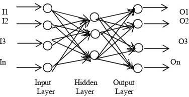
Back-propagation algorithm [7] is a widely used learning algorithm in Artificial Neural Networks. The Feed-Forward Neural Network architecture (Fig. 1) is capable of approximating most problems with high accuracy and generalization ability. This algorithm is based on the error-correction learning rule. Error propagation consists of two passes through the different layers of the network, a forward pass and a backward pass. In the forward pass the input vector is applied to the sensory nodes of the network and its effect propagates through the network layer by layer. Finally a set of outputs is produced as the actual response of the network. During the forward pass the synaptic weight of the networks are all fixed. During the back pass the synaptic weights are all adjusted in accordance with an error-correction rule. The actual response of the network is subtracted from the desired response to produce an error signal. This error signal is then propagated backward through the network against the direction of synaptic conditions. The synaptic weights are adjusted to make the actual response of the network move closer to the desired response.
I1 O1
I2 O2
I3 O3
In On Input Hidden Output
Layer Layer Layer
Fig. 1 Feed-Forward Neural Network Architecture
A. Algorithm
Step 1: Normalize the inputs and outputs with respect to their maximum values. It is proved that the neural networks work better if input and outputs lie between 0-1. For each training pair, assume there are ‘I’ inputs given by
{I} I and ‘n’ out puts {o} o in a normalized form.
l x 1 n x 1
Step2: Assume the number of neurons in the hidden layer to lie between l<m<2l
Step3: [v] represents the weights of synapses connecting Input neurons and hidden neurons and [w] represents weights of synapses connecting hidden neurons and output neurons. Initialize the weights to small random values usually from -1 to 1.For general problems, λ can be assumed as 1 and the threshold values can be taken as zero.
[v]o = [random weights] [w]o = [random weights]
[∆v]o = [∆w]o =[o]
Step4: For the training data, present one set of inputs and outputs. Present the pattern to the input layer as inputs to the input layer. By using linear activation function, the output of the input layer may be evaluated as
{o}r = {r}r (1)
l x 1 l x 1
Step 5: Compute the inputs to the hidden layer by multiplying corresponding weights of synapses as
{I}H = [V]T {O}r (2)
m x 1 m x l l x 1
Step6: Let the hidden layer units evaluate the output using the sigmodial function as
(3) Step7: Compute the inputs to the output layer by multiplying corresponding weights of synapses as
{I}o = [W] T{o}H (4)
n x 1 n x m m x 1
(5) The above is the network output.
Step9: Calculate the error and the difference between the network output and the desired output as for the ith training set as
(6) Step10: Find {d} as
(7)
Step 11: Find [Y] matrix as
[Y] = {o}H <d> (8)
m x n m x 1 1 x n
Step 12: Find [∆w]t+1 = α [∆w]t + η[Y] (9) m x n m x n m x n
Step 13: Find {e} = [w] {d} (10) m x 1 m x n n x 1
{d*} =
m x 1 m x 1
(11) Find [X] matrix as
[X] = {O} I <d*> = {I}I <d*> (12)
1 x m 1 x 1 1 x m 1 x 1 1 x m
Step 14: Find [∆v]t+1 = α [∆v]t + η[X] (13) 1 x m 1 x m 1 x m
Step 15: Find [v]t+1 = [v]t + [∆v]t + 1 (14) [w]t+1 = [w]t + [∆w]t + 1 (15)
Step 16: Find error rate as ∑Ep
Error rate =
nset (16) Step 17: Repeat steps 4 -16 unit the convergence in the error rate is less than the tolerance value.
B. Procedure for Image Compression
The image is split into non-overlapping sub-images. Say for example 256 x 256 bit image will be split into 4 x 4 or 8 x 8 or
16 x 16 pixels. The normalized pixel value of the sub-image will be the input to the nodes. The three-layered back propagation-learning network will train each sub-image. The number of neurons in the hidden layer will be designed for the desired compression. The number of neurons in the output layer will be the same as that in the input layer. The input layer and output layer are fully connected to the hidden layer. The Weights of synapses connecting input neurons and hidden neurons and weight of synapses connecting hidden neurons and weight of synapses connecting hidden neurons and output neurons are initialized to small random values from say –1 to +1.The output of the input layer is evaluated using linear activation function. The input to the hidden layer is computed by multiplying the corresponding weights of synapses. The hidden layer units evaluate the output using the sigmoidal function. The input to the output layer is computed by multiplying the corresponding weights of synapses. The output layer neuron evaluates the output using sigmoidal function. The Mean Square error of the difference between the network output and the desired output is calculated. This error is back propagated and the weight synapses of output and input neurons are adjusted. With the updated weights error is calculated again. Iterations are carried out till the error is less than the tolerance. The compression performance is assessed in terms of Compression ratio, PSNR and execution time [8].
III. MAPPING OF PIXELS BY ESTIMATING THE CUMULATIVE DISTRIBUTION FUNCTION OF THE IMAGE
Computational complexity is involved in compression of raw pixels of an image in spatial domain or the mathematically transformed coefficients in frequency domain using Artificial Neural Networks. The efficiency of such Artificial Neural Networks is pattern dependent. An image may contain a number of distinct gray levels with narrow difference with their neighborhood pixels. If the gray levels of the pixels in an image and their neighbors are mapped in such a way that the difference in the gray levels of the neighbor with the pixel is minimum, then compression ratio as well as the convergence of the network can be improved. To achieve this, the Cumulative Distribution Function [9] is estimated for the image and it is used to map the image pixels. When the mapped image pixels are used, the Back-propagation Neural Network yields high compression ratio as well as it converges quickly.
Consider an image as a collection of random variables, each with cumulative distribution and density of
Fx (x) = Prob {X ≤ x} (17)
d
px (x) = dx Fx (x) (18)
Now consider forming the following random variable.
Y = Fx (x) (19)
Here Y is the result of mapping the random variable x through its own Cumulative Distribution Function. The cumulative distribution of Y can be easily computed.
Fy (y)= Prob {Fx(x) ≤ y}
•
•
ei (OHi) (1-OHi)
•
= Prob {X≤ Fx-1(y)}
= Fx (Fx-1(y))
0 for y < 0 = y for 0 ≤ y ≤ 1
1 for y > 1 (20) This shows that y has a uniform distribution on the interval
(0,1) Therefore the histogram of an image can be equalized by mapping the pixels through their cumulative distribution function Fx (x). In order to implement histogram equalization,
the cumulative distribution function for the image is estimated. It is done using the image histogram. Let h(i) be the histogram of the image formed by computing the number of pixels at gray level i. Typically, the pixels take on the values i=0, …,L-1 where L = 256 is the number of discrete levels that a pixel can take on. The cumulative distribution function can then be approximated by
1 j=1
Fx(i) = ∑ h (j) (21)
h(L-1) j=0
Here the normalization term assures that Fx(L-1)=1. By
applying the concept of equation (17), a pixel of Xs is
equalized at the position s Є S where S is the set of position in the image.
Ys= Fx (Xs) (22)
However, Ys has a range from 0 to 1 and may not extend over
the maximum number of gray levels. To correct these problems, we first compute the minimum and maximum values of Ys.
Ymax = max Ys (23) sЄЅ
Ymin = min s Є SYs (24)
And then we use these values to from Zs, a renormalized
version of Ys
Fx(Xs) - Ymin
Zs = (L-1) Ymax - Ymin (25)
The transformation form Xs to Zs. is Histogram
Equalization.
Histogram equalization does not introduce new intensities in the image. Existing values will be mapped to new values resulting image with less number of the original number of intensities. Mapping of the pixels by estimating the cumulative Distribution function of the image results in correlation of the pixels and the presence of similar pixel values within the small blocks of image augments the convergence of the network. Further the frequency of occurrence of gray levels in the image will be more are less equal or rather uniform by the mapping .Due to this most of the image blocks will be similar and hence the learning time gets reduced. Since the convergence is quick, it is possible to reduce the number of neurons in the hidden layer to the minimum possible thus achieving high compression ratios without loss in quality of the decompressed image. The quality of the decompressed image and the convergence time
has been experimentally proved to be better than achieved by conventional methods and by the same algorithm without mapping the image by Cumulative Distribution function. The correlation of pixel values plays a vital role in augmenting the convergence of the neural network for image compression and this is a simple mechanism compared to other existing transformation methods, which are computationally complex and lengthy process.
IV. EXPERIMENTAL RESULTS
V. CONCLUSION
The Back Propagation Neural Network has the simplest architecture of the various Artificial Neural Networks that have been developed for Image Compression. The direct pixel based manipulation, which is available in the field of Image Compression, is still simpler. But the drawbacks are very slow convergence and pattern dependency. Many research works have been carried out to improve the speed of convergence. All these methods are computationally complex in nature, which could be applied only to limited patterns. The proposed approach of mapping the pixels by estimating the Cumulative Distribution Function is a simple method of pre-processing any type of image. Due to the uniform frequency of occurrence of gray levels by this optimal contrast stretching, the convergence of the Back-Propagation Neural Network is augmented. There will not be any loss in data in the pre-processing and hence the finer details in the image are preserved in the reconstructed image. However since the original intensities will be mapped to new values, re-transformation of the Decompressed image is suggested in case of Medical Images.
(a) (b) (c) Fig. 2 Standard Image
(a) Original image (b) Mapped by CDF (c) Decompressed PSNR = 28.91dB, Convergence Time = 182 Sec.
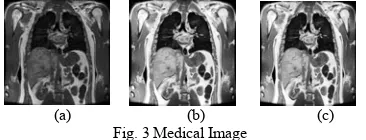
(a) (b) (c) Fig. 3 Medical Image
(a) Original image (b) Mapped by CDF (c) Decompressed PSNR = 29.42dB, Convergence Time = 140 Sec.
(a) (b) (c) Fig. 4 Satellite Image
(a) Original image (b) Mapped by CDF (c) Decompressed PSNR = 29.11dB, Convergence Time = 160 Sec.
TABLEI
EXPERIMENTAL RESULTS OF THE PROPOSED APPROACH
S.No Image CR PSNR
(dB)
TIME (Sec)
1 Cameraman 4.1 29.78 148
2 Lena 4:1 28.91 182
3 Pepper 4:1 29.04 188
4 Fruits 4:1 29.79 185
5 Boat 4:1 29.12 178
6 Mandrill 4:1 29.68 161 7 Abdomen(Mri) 4:1 29.42 140 8 Thorax(Mri) 4:1 29.61 132 9 Satellite 4:1 29.11 160
TABLEII
EXPERIMENTAL RESULTS WITHOUT MAPPING
REFERENCES
[1] M.Egmont-Petersen, D.de.Ridder, Handels, “Image Processing with Neural Networks – a review”, Pattern Recognition 35(2002) 2279-2301, www.elsevier.com/locate/patcog
[2] Bogdan M.Wilamowski, Serdar Iplikci, Okyay Kaynak, M. Onder Efe “An Algorithm for Fast Convergence in Training Neural Networks”. [3] Fethi Belkhouche, Ibrahim Gokcen, U.Qidwai, “Chaotic gray-level
image transformation, Journal of Electronic Imaging -- October - December 2005 -- Volume 14, Issue 4, 043001 (Received 18 February 2004; accepted 9 May 2005; published online 8 November 2005. [4] Hahn-Ming Lee, Chih-Ming Cheb, Tzong-Ching Huang, “Learning
improvement of back propagation algorithm by error saturation prevention method”, Neurocomputing, November 2001.
[5] Mohammed A.Otair, Walid A. Salameh, “Speeding up Back-propagation Neural Networks” Proceedings of the 2005 Informing Science and IT Education Joint Conference.
[6] M.A.Otair, W.A.Salameh (Jordan), “An Improved Back-Propagation Neural Networks using a Modified Non-linear function”, The IASTED Conference on Artificial Intelligence and Applictions, Innsbruck, Austria, February 2006.
[7] Simon Haykin, “Neural Networks – A Comprehensive foundation”, 2nd
Ed., Pearson Education, 2004.
[8] B.Verma, B.Blumenstin and S. Kulkarni, Griggith University, Australia, “A new Compression technique using an artificial neural network”. [9] Rafael C. Gonazalez, Richard E.Woods, “Digital Image Processing”, 2nd
Ed., PHI, 2005. S.No
Image CR PSNR
(dB)
TIME (Sec)
1 Cameraman 4:1 26.89 320
2 Lena 4:1 26.11 365
3 Pepper 4:1 26.52 368
4 Fruits 4:1 26.96 361
5 Boat 4:1 26.75 342